2. FUNDAMENTALS OF THE STANDARD COSMOLOGY

2.1. Homogeneity and Isotropy: The Robertson-Walker Metric

Cosmology as the application of general relativity (GR) to the entire universe would seem a hopeless endeavor were it not for a remarkable fact - the universe is spatially homogeneous and isotropic on the largest scales.

"Isotropy" is the claim that the universe looks the same in all direction. Direct evidence comes from the smoothness of the temperature of the cosmic microwave background, as we will discuss later. "Homogeneity" is the claim that the universe looks the same at every point. It is harder to test directly, although some evidence comes from number counts of galaxies. More traditionally, we may invoke the "Copernican principle," that we do not live in a special place in the universe. Then it follows that, since the universe appears isotropic around us, it should be isotropic around every point; and a basic theorem of geometry states that isotropy around every point implies homogeneity.

We may therefore approximate the universe as a spatially homogeneous and isotropic three-dimensional space which may expand (or, in principle, contract) as a function of time. The metric on such a spacetime is necessarily of the Robertson-Walker (RW) form, as we now demonstrate. ⁽¹⁾

Spatial isotropy implies spherical symmetry. Choosing a point as an origin, and using coordinates (r, , ) around this point, the spatial line element must take the form

(1)

where f (r) is a real function, which, if the metric is to be nonsingular at the origin, obeys f (r) ~ r as r 0.

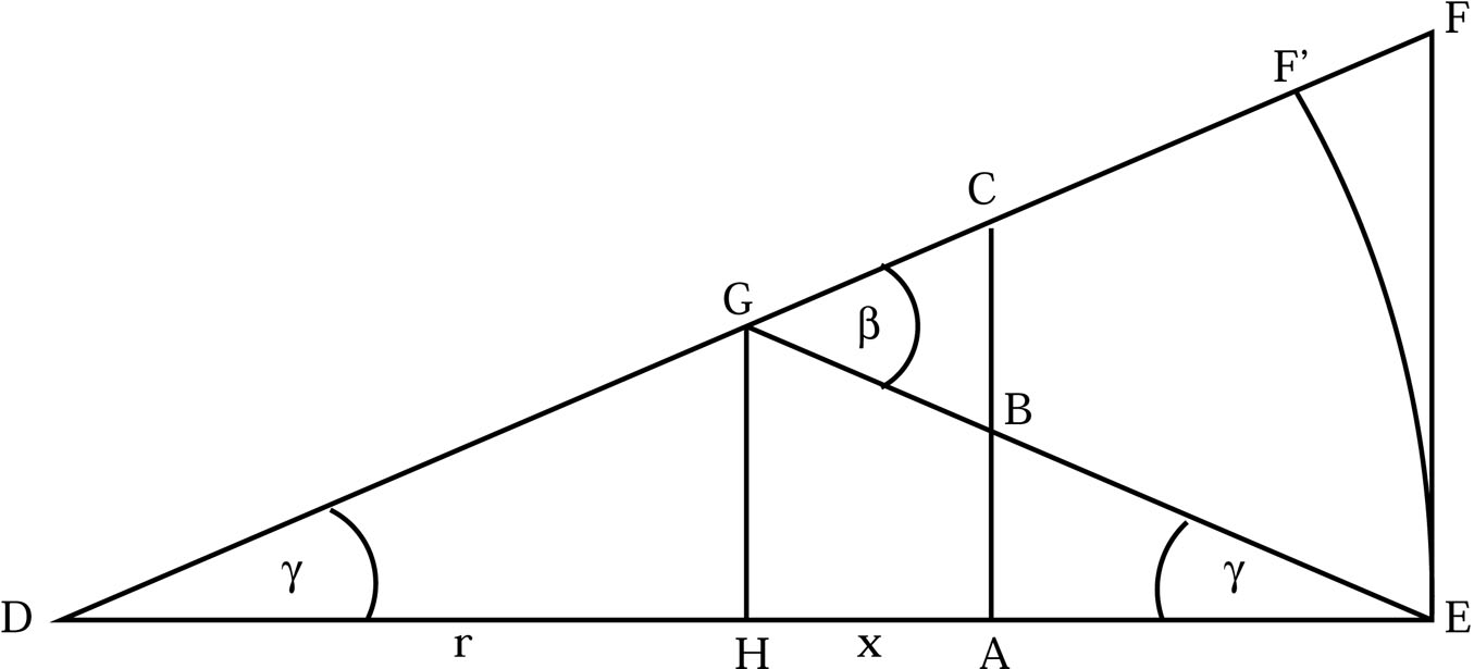Figure 2.1. Geometry of a homogeneous and isotropic space.

Now, consider figure 2.1 in the = /2 plane. In this figure DH = HE = r, both DE and are small and HA = x. Note that the two angles labeled are equal because of homogeneity and isotropy. Now, note that

(2)

Also

(3)

Using (2) to eliminate / , rearranging (3), dividing by 2x and taking the limit x yields

(4)

We must solve this subject to f (r) ~ r as r 0. It is easy to check that if f (r) is a solution then f (r / ) is a solution for constant . Also, r, sin r and sinh r are all solutions. Assuming analyticity and writing f (r) as a power series in r it is then easy to check that, up to scaling, these are the only three possible solutions.

Therefore, the most general spacetime metric consistent with homogeneity and isotropy is

(5)

where the three possibilities for f () are

(6)

This is a purely geometric fact, independent of the details of general relativity. We have used spherical polar coordinates (, , ), since spatial isotropy implies spherical symmetry about every point. The time coordinate t, which is the proper time as measured by a comoving observer (one at constant spatial coordinates), is referred to as cosmic time, and the function a(t) is called the scale factor.

There are two other useful forms for the RW metric. First, a simple change of variables in the radial coordinate yields

(7)

where

(8)

Geometrically, k describes the curvature of the spatial sections (slices at constant cosmic time). k = + 1 corresponds to positively curved spatial sections (locally isometric to 3-spheres); k = 0 corresponds to local flatness, and k = - 1 corresponds to negatively curved (locally hyperbolic) spatial sections. These are all local statements, which should be expected from a local theory such as GR. The global topology of the spatial sections may be that of the covering spaces - a 3-sphere, an infinite plane or a 3-hyperboloid - but it need not be, as topological identifications under freely-acting subgroups of the isometry group of each manifold are allowed. As a specific example, the k = 0 spatial geometry could apply just as well to a 3-torus as to an infinite plane.

Note that we have not chosen a normalization such that a₀ = 1. We are not free to do this and to simultaneously normalize | k| = 1, without including explicit factors of the current scale factor in the metric. In the flat case, where k = 0, we can safely choose a₀ = 1.

A second change of variables, which may be applied to either (5) or (7), is to transform to conformal time, , via

(9)

Applying this to (7) yields

(10)

where we have written a() a[t()] as is conventional. The conformal time does not measure the proper time for any particular observer, but it does simplify some calculations.

A particularly useful quantity to define from the scale factor is the Hubble parameter (sometimes called the Hubble constant), given by

(11)

The Hubble parameter relates how fast the most distant galaxies are receding from us to their distance from us via Hubble's law,

(12)

This is the relationship that was discovered by Edwin Hubble, and has been verified to high accuracy by modern observational methods (see figure 2.2).

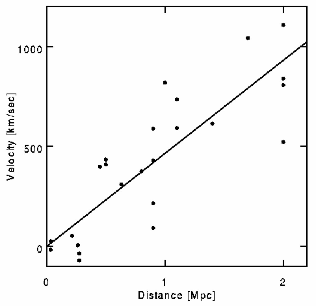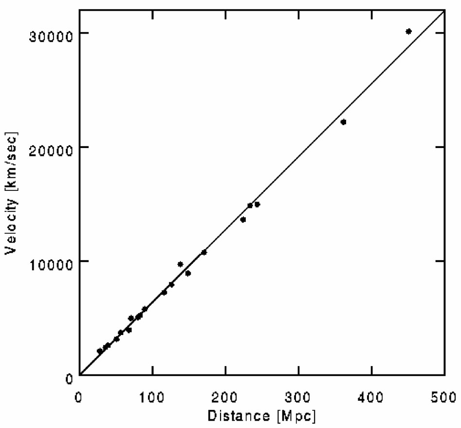Figure 2.2. Hubble diagrams (as replotted in [17]) showing the relationship between recessional velocities of distant galaxies and their distances. The left plot shows the original data of Hubble [18] (and a rather unconvincing straight-line fit through it). To reassure you, the right plot shows much more recent data  [19], using significantly more distant galaxies (note difference in scale).

¹ One of the authors has a sentimental attachment to the following argument, since he learned it in his first cosmology course [16]. Back.