1.5. Interferometric techniques

The technique of interferometry was originally developed with the intention of achieving high angular resolution, and instruments such as the VLA are examples of this. The SZ effect is primarily a large angular-scale feature on the sky, so high resolution is not of interest and is, in fact, detrimental in this context. However, interferometers offer improvements in the control of systematic effects compared with single-dish telescopes. First, interferometers experience a loss of coherence (and thus a loss of sensitivity) away from the pointing centre, meaning that ground spillover, terrestrial interference and other spurious signals will be attenuated. Second, structures on the sky are modulated by a fringe pattern at a different rate than most contaminating sources. This allows rejection of signals from astronomical sources such as the Sun and bright planets. Finally, interferometers with a wide range of baselines allow simultaneous observations of confusing, small angular-scale, possibly-variable radio sources, so that their effects can be separated from the SZ signal.

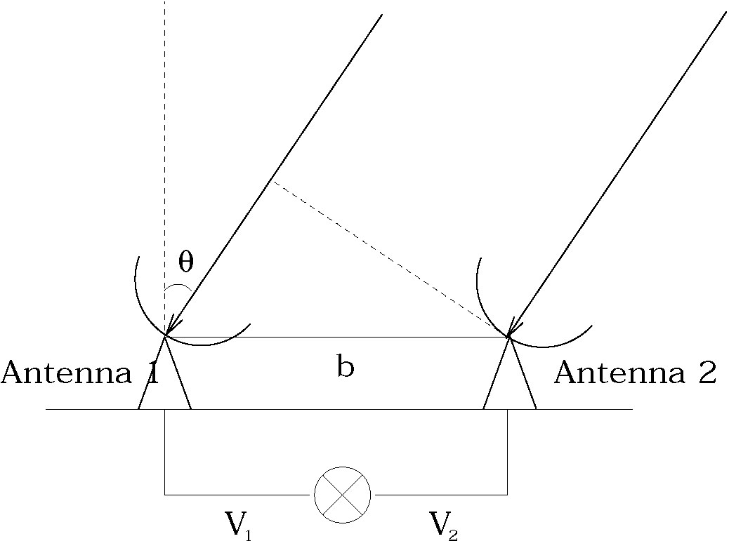Figure 4. A simple one-dimensional interferometer. Radiation from the source must travel an extra distance b sin to reach antenna 1.

We can understand the basic principles of interferometry by discussion of a simple case. Consider a two-element interferometer, with antennas separated by a distance b, observing a source at an angle , as shown in Fig. 4. Each antenna receives a signal which produces a time-varying voltage, and the product of these voltages is measured. Due to the path difference for radiation travelling from a distant source to the two antennas, there will be a phase difference between the received signals given by

(12)

The correlated output is then

(13a) (13b)

In practice the output is integrated over some time interval so that the rapidly-varying second and third terms average to zero. If the energy received from the source per unit area is S, and the area of each antenna is a, the interferometer response is

(14)

Phases are usually not measured absolutely, but relative to some reference direction, ₀. For a source offset by a small angle from ₀, we have = ₀ + and (14) becomes

(15a) (15b)

since we are dealing with small angles. The correlated output differs at different antenna separations, so that the angular resolution of this simple interferometer is proportional to / b. A more complex multi-baseline instrument is sensitive to a range of scales determined by the set of baseline lengths defined by the antenna locations. The shortest baseline defines the maximum scale which can be sampled. Sky structures on larger angular scales will not modulate with ₀ (and hence with time), and so will not produce a detected signal.

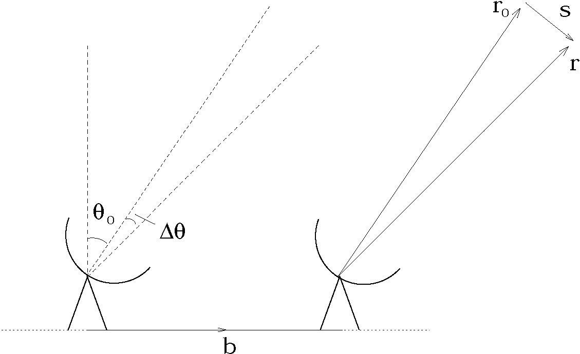Figure 5. The same simple interferometer as Fig. 4, where the field centre is specified by r0 and the source position is r. 0 and are the angles discussed in the text.

The interferometer response can be expressed more generally -- we consider the main points here, but a full treatment is given in Thompson, Moran and Swenson (1986). If we now specify the source position by a vector r (see Fig. 5) and the baseline by the vector b, the phase difference from (12) can be written = (2 / ) b.r. The reference direction may be specified by a vector r₀, so that r = r₀ + s, where s describes the shift between the two. After some manipulation, the response to all sources within the solid angle becomes

(16)

It is conventional to specify the baseline vector b in terms of right-handed coordinates (u, v, w), where w is in the direction of the source, u and v point East and North respectively as seen from the source position, and distances are measured in wavelengths. Additionally, the position of the source on the sky is usually described in terms of co-ordinates (l, m, n). We see that b.r₀ = w, and b.r = (ul + vm + wn) , thus b.s = (ul + vm + w(n - 1)) . Making the substitution d = (dl dm) / n, we find

(17)

where a(l, m) is the effective total area of the antennas in the direction (l, m) and I(l, m) is the brightness distribution on the sky. n = (1 - l² - m²)^1/2 1 for small angles, simplifying the Fourier inversion required in eq. (17) to produce a sky map of I(l, m). A map made from interferometer data contains structures which are modulated by the synthesized beam. This is given by the Fourier transform of the telescope aperture, which is eq (17) above with the sky brightness replaced by a two-dimensional function.