


2.6. Cluster Hubble diagram
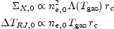
One of the major uses to which the thermal SZ effect has been put is that of determining the Hubble constant. In its simplest form, the method is to compare the X-ray surface brightness and the thermal SZ effect at the centre of a cluster
 |
(32a) (32b) |
where rc is some measure of the scale of the cluster
(often the core radius of the best-fitting isothermal
 model), and the
constants of proportionality include factors from the shapes of the
distributions of electron density and electron temperature. The X-ray
emissivity of the gas,
model), and the
constants of proportionality include factors from the shapes of the
distributions of electron density and electron temperature. The X-ray
emissivity of the gas,  (Tgas), is here taken to be a
constant over the atmosphere, assuming that the cluster is isothermal
and has a constant metal abundance. Then the combination
(Tgas), is here taken to be a
constant over the atmosphere, assuming that the cluster is isothermal
and has a constant metal abundance. Then the combination
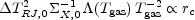 |
(33) |
and a measure of the angular size of the cluster,
 c,
can be compared with the linear size, rc, to derive
the angular diameter distance of the cluster
c,
can be compared with the linear size, rc, to derive
the angular diameter distance of the cluster
 |
(34) |
An example of the application of this method is given in Sec. 3, but it is clear from eq. (33) that errors in the SZ effect and X-ray temperature have a major impact on the accuracy of the angular diameter distance that is derived. Although the angular diameter distances derived in this way can be used to construct a "cluster Hubble diagram" of angular diameter distance as a function of redshift (Birkinshaw 1999; Carlstrom et al. 2002), and in principle this diagram could be used to deduce further cosmological parameters than the Hubble constant, the errors on the distance estimates are currently too large to make this possible.
Clearly a major requirement for the use of this method is that the
thermal SZ effect and the X-ray brightness of the cluster are accurately
determined: the dominant error is from the SZ effect, since a 5%
systematic error in the flux density scale of the SZ effect
(Sec. 2.1.1) leads to a 10% error in the
distance scale.
However, if the Hubble constant itself is not of interest, but rather
the intention is to use the Hubble diagram to estimate the density
parameters
( m 0,
0),
then the absolute
calibration not important -- it represents merely a shift of the
overall distance scale -- and only the shape of the angular diameter
distance/redshift relation is important.
m 0,
0),
then the absolute
calibration not important -- it represents merely a shift of the
overall distance scale -- and only the shape of the angular diameter
distance/redshift relation is important.
The large-scale model of the cluster gas (Sec. 2.2.2) determines the constant of proportionality in eq. (34), and so it is essential that a correct model is adopted. Since the X-ray data are sensitive to emission from the inner part of the cluster, while the SZ data are relatively more sensitive in the outer regions (because of the different ne scalings), a high-sensitivity X-ray image of the cluster is essential to trace the gas out to sufficient distance that the model can be used with confidence.
On the smallest angular scales, below the angular resolution of the X-ray image, the gas may be significantly clumped because of the effects of turbulence induced by galaxies moving at transonic speeds, the dissipation of gas from infalling groups, local heating from low-power radio sources, etc. Such clumping has a significant effect on the constant of proportionality in eq. (34). For example, if the clumping is isothermal, then the clumping factor
 |
(35) |
measures the excess of X-ray emissivity over that obtained from a smooth density distribution, and the distance inferred by assuming that the density distribution is smoothed and unclumped is an underestimate by a factor C. Limits to the amount of non-isothermal clumping can be deduced from the detailed X-ray spectrum of a cluster, if the spectrum contains enough counts, but limits on the amount of isothermal clumping can only be based on theoretical considerations about the dissipation time of the implied overpressure and the rate of creation of the clumps.
This issue may induce not only a scale error in the Hubble diagram,
and hence an error in the Hubble constant, but could also change the
shape of the diagram if the average dynamical state of the
intracluster medium evolves with time -- perhaps from a clumpy
initial state, just after the atmosphere assembles, into a smoother
and more relaxed state at the present time. Thus the uncritical use of
the cluster Hubble diagram may lead to significant errors in the
estimation of the cosmological parameters
(m 0,
0)
that dictate how the angular diameter distance changes with redshift.
Eq. (34) derives the angular diameter distance for a cluster by comparing its line-of-sight scale with its transverse angular size. If the cluster is non-spherical, then this ratio will not yield the angular diameter distance correctly. However, if a sample of clusters at similar redshifts, with random orientations, is used, then an average over this sample with its various cluster shapes should reduce the error, at the expense of adding substantially to the noise in the distance estimate.
Such an average will not be successful if the set of clusters is biased, and a bias is likely for the faintest clusters since non-spherical atmospheres have higher central surface brightnesses, and so are easier to detect, if their long axes lie close to the line of sight. It is, therefore, important to select a sample of clusters that has no orientation bias. This can be done either by selecting clusters which are far above the surface brightness limit of some finding survey, or by selecting clusters based on an integrated, surface-brightness independent, indicator of cluster properties. An ideal selection would be the integrated thermal SZ effect, since this is a linear indicator of the total electron count in a cluster, and so is orientation independent.