


This section concentrates on derivatives from the observations and their possible interpretations. Recent years have seen several variations emerging from the formerly very uniform picture. The original assertion that all SNe Ia are the same had to be abandoned as better data became available. In particular, the strong belief in the standard candle picture, so important for the cosmological applications of SNe Ia, has been overthrown by large deviations in light curve shape and spectral appearance. The monolithic picture of SNe Ia has been replaced by several correlations of observable parameters. The full extent of these correlations has not yet been explored and new ones are still uncovered.
One of the key questions will be whether SN 1991bg represents an extreme case in the SN Ia picture or whether it should be considered separate and independent of the majority of Ia events. Specifically, it would be interesting to see whether this object underwent a fundamentally different explosion (maybe still in the realm of the thermonuclear explosions) or whether it represents a stripped version of the regular explosions.
Despite their differences SNe Ia seem to follow a few invariants in
their appearance. The best-known is the linear decline-rate vs.
luminosity correlation
(Phillips 1993).
There are now several implementations of this
correction: the template fitting or
 m15
method
(Hamuy et al. 1996b,
Phillips et
al. 1999),
the multi-light curve shape correction
(Riess et al. 1996a,
1998a),
and the stretch factor
(Perlmutter et
al. 1997).
Earlier versions of such light curve shape vs. luminosity relations
had been proposed
(Barbon et al. 1973a,
Pskovskii 1977,
1984),
but could not be supported by the available data.
m15
method
(Hamuy et al. 1996b,
Phillips et
al. 1999),
the multi-light curve shape correction
(Riess et al. 1996a,
1998a),
and the stretch factor
(Perlmutter et
al. 1997).
Earlier versions of such light curve shape vs. luminosity relations
had been proposed
(Barbon et al. 1973a,
Pskovskii 1977,
1984),
but could not be supported by the available data.
The decline rate correction methods are entirely empirical. They rely on the fact that the fit around the Hubble line in the Hubble diagram improves when they are applied. Originally based on a set of supernovae with known relative distances a linear relation for the decline in the B light curves and the B, V, and I filter luminosities was determined (Phillips 1993). It has to be stressed that the relation is normally defined for the decline in the B filter light curve. The coefficients of this relation have changed significantly over the last few years as the distances and extinction corrections have been refined (Hamuy et al. 1996c, Phillips et al. 1999; Riess et al. 1996a, 1998a). Higher order fits have now been proposed (Riess et al. 1998a, Phillips et al. 1999, Saha et al. 1999). The stretch factor method describes the light curves by a simple stretch in time. A basic template light curve is used and then stretched to match the observations (Perlmutter et al. 1997). This method only works for the B and V light curves through the peak phase, but breaks down about 4 weeks after peak. It is clear from the R and I light curve shapes that such a stretching procedure can not work linearly for all filters. Another potential problem with this method is that it predicts the relative times between filter maxima to stretch as well, which is not observed. Within these limitations it has been shown that the stretching provides similar corrections as the other methods discussed above (Perlmutter et al. 1997; but see below).
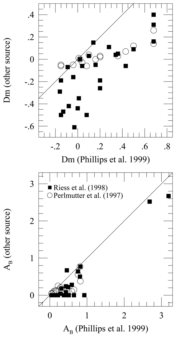
Although some of the methods are equivalent they do not reproduce too well. An example is given in Figure 4 (top) which shows the magnitude corrections determined by the three methods for the same supernovae. For the construction of this diagram we have calculated the magnitude correction given in Phillips et al. (1999) for the template method. The values for MLCS have been taken from Table 10 in Riess et al. (1998a) and the stretch correction derived from Table 2 in Perlmutter et al. (1999). Note that the assumptions for these magnitude corrections are not identical for all methods. While Phillips et al. (1999) used BVI light curves for their corrections, the ones by Riess et al. (1998a) and Perlmutter et al. (1999) are based on B and V only. A significant scatter is noticeable. There is also a significant zero-point offset of 0.25 ± 0.04 magnitudes for the MLCS method, while the stretch yields only a marginal offset of -0.03 ± 0.01 mag. The slopes are further 0.77 ± 0.13 and 0.29 ± 0.04 for MLCS and stretch, respectively. These are significantly different from the one expected, if the methods were identical. The scatter is considerable and also a concern. A similar conclusion can be drawn from the comparison of the estimated absorption towards the supernovae (Fig. 4 bottom). The data are from the same sources as the magnitude corrections. In particular, the large spread of absorptions from the template method compared to both MLCS and stretch determinations (which are based on B and V only for these data here) is striking. An overall offset is apparent here as well. These are all signatures of subtle, but significant differences in the treatment of the data. A similar conclusion has been drawn in connection with data for distant SNe Ia (Drell et al. 1999), but attributed to evolution.
|
Figure 4. Comparison of the light curve
parameters from different methods. The multi light curve shape
(Riess et al. 1998a)
and the stretch corrections
(Perlmutter et
al. 1997)
are compared to the template
( |
The main differences are related to the exact correction for dust in the host galaxy. The determination of the extinction relies on the availability of an independent absorption indicator. In fact, the reddening law in most cases has to be assumed instead of being derived (for exceptions see Riess et al. 1996b who find a slight deviation from the Galactic reddening law and Phillips et al. (1999) who don't). The best that could be done in the past was to assume that SNe Ia all have the same (Branch & Tammann 1992 and discussion therein) or a well-defined color (Riess et al. 1996a) at maximum. With this assumption and the application of the Galactic reddening law, absorptions could be measured. Phillips et al. (1999) recently proposed to use the color at the transition to the nebular phase at an epoch of about 30 days past peak rather than the color at maximum. At the transition all supernovae are at about the same epoch since explosion and the various iron-element emission lines, which dominate the spectrum, have the same relative strengths. The peak colors depend on the exact changes of the optical depth in the ejecta. The color evolution at maximum is also very rapid and small measurement errors can result in systematically wrong reddening estimates.
An attempt has been made to combine the known relations into a method for distance determinations from minimal observations (Riess et al. 1998b). With a single spectrum during the peak phase and photometry at one epoch in at least two filters the absolute luminosity and the peak brightness of the event can be determined. The spectrum in this case provides the information of the phase/age of the supernova and, through the line strengths, the 'luminosity class,' while the reddening and brightness are determined from the photometry. The assumption in all this is, of course, that all SNe Ia can be described in a single parameter family and the reddening law is well understood.
An independent fitting method has been applied by Vacca & Leibundgut (1996, 1997) and Contardo et al. (2000). Here the data are approximated with a function which depends on a number of parameters. This fitting method also reproduces the decline rates found by other methods (Vacca & Leibundgut 1997). Its application to larger data sets is still missing, but would provide a strong independent check on the relations.
There are other parameters which correlate with the peak luminosity of SNe Ia. They are the rise time to maximum (Riess et al. 1999b), color near maximum light (Riess et al. 1996a, Tripp 1998, Phillips et al. 1999), line strengths of Ca and Si absorption lines (Nugent et al. 1995, Riess et al. 1998b), the velocities as measured in Fe lines at late phases (Mazzali et al. 1998), the host galaxy morphology (Filippenko 1989, Hamuy et al. 1996a, Schmidt et al. 1998), and host galaxy colors (Hamuy et al. 1995, Branch et al. 1996). There may be indications that the secondary peak in the I light curves and also the shoulder in the bolometric light curves correlate with the absolute luminosity (Hamuy et al. 1996d, Riess et al. 1999a, Contardo et al. 2000).
The observable emission of SNe Ia is powered completely by the decay of
radioactive 56Ni and its radioactive daughter nucleus
(Colgate & McKee
1969,
Clayton 1974).
56Ni is synthesized in the explosion and
decays by electron capture with a half-life of 6.1 days to 56Co.
The cobalt decays through electron capture (81%) and
 +
decay (19%) to stable 56Fe with a half-life of 77 days.
The early phase is dominated by the down-scattering
and the release of photons generated as
+
decay (19%) to stable 56Fe with a half-life of 77 days.
The early phase is dominated by the down-scattering
and the release of photons generated as
 -rays in
the decays
(Höflich et
al. 1996,
Eastman 1997,
Pinto & Eastman
2000).
The dominating opacity comes from the strongly velocity broadened lines and
the incoherent scattering ('line splitting').
-rays in
the decays
(Höflich et
al. 1996,
Eastman 1997,
Pinto & Eastman
2000).
The dominating opacity comes from the strongly velocity broadened lines and
the incoherent scattering ('line splitting').
At late phases the optical radiation is escaping freely and the ejecta
are cooling through emission lines. The
-ray
escape fraction increases continually and less and less energy is
converted to optical photons
(Leibundgut & Pinto 1992).
After about 150 days
the contribution from positrons becomes significant
(Axelrod 1980,
Milne et al. 1999).
These positrons
are from a minor channel of the 56Co decay and annihilate in the
ejecta after losing their kinetic energy in elastic scatterings
(Axelrod 1980,
Leibundgut &
Pinto 1992,
Ruiz-Lapuente et
al. 1995b,
Milne et al. 1999).
So far it had been assumed that all the energy from the positron decay
would be deposited in the ejecta, but recent studies indicate that
depending on the magnetic field structure in the ejecta some positrons
could escape and the decay energy is lost for the supernova
(Colgate et al. 1980,
Ruiz-Lapuente &
Spruit 1998,
Milne et al. 1999).
After several hundred days the emission should change dramatically when the ejecta has cooled down far enough that the bulk of the cooling occurs through far-infrared fine structure lines of iron (Fransson et al. 1996). This has so far not been observed in any SN Ia as they are too faint at this point. In some cases the emission becomes dominated by light echos (e.g. 1991T: Schmidt et al. 1994, Boffi et al. 1999).
All inference of the progenitor systems of supernovae has to come from the explosion observations themselves. The name of the game is to match stellar evolution models with some parameters indirectly derived from the explosions. Excellent reviews of this topic are available (Branch et al. 1995, Renzini 1996, Livio 1999, Nomoto 1999) and we refer the reader to the references in these compilations.
The observations of SNe Ia tell us that they emerge from a compact
object as is inferred from the light curves, i.e. the short duration of
the peak phase. The fast decline and the large leakage of
-rays,
although only measured indirectly, imply a small mass of the ejecta as well.
Note that this statement implicitly made use of the thermonuclear explosion
models (cf. Section 4).
The glaring absence of the most abundant elements in the universe,
hydrogen and helium, narrow the selection down to a few highly evolved
objects. Also the appearance in elliptical galaxies with their old
stellar population hints at significant nuclear processing before
explosion.
Indirectly these observational results indicate that SNe Ia do not
emerge from single star systems. The absence of hydrogen and helium must
mean that the star has removed its envelope. The longevity of the
progenitors, at least for SNe Ia in elliptical galaxies, and the
trigger of the explosion also point to binary systems.
An important piece of information is the rarefied environment in which
SNe Ia
explode. Radio emission is the telltale signature of such circumstellar
material, but has not been detected in a single SN Ia. This also sets
limits on mass-loss from companion stars. A potentially powerful
analysis tool would be the detection of narrow
H or He emission from
gas shed by the companion star. The best observations to test for such
emission have been obtained for SN 1994D without a detection
(Cumming et al. 1996).
The investigation of local interstellar
environments of SNe Ia has so far been inconclusive
(Van Dyk et
al. 1999),
but there are at least four cases which could lie close or within
an area of active star formation.
or He emission from
gas shed by the companion star. The best observations to test for such
emission have been obtained for SN 1994D without a detection
(Cumming et al. 1996).
The investigation of local interstellar
environments of SNe Ia has so far been inconclusive
(Van Dyk et
al. 1999),
but there are at least four cases which could lie close or within
an area of active star formation.
The rareness of SNe Ia is a further indicator of a special stellar evolution scenario leading to these explosions. With so few stars producing SNe Ia the selection criterion must be rather severe.
The uniform appearance is often used as an argument for a restrictive progenitor base, but in the light of the recent observations, in particular of the faint objects SN 1991bg and SN 1997cn, this should be investigated again carefully. On the other hand, the strong correlations hint at fairly unique progenitor systems allowing for some variations.
Most discussions on SN Ia progenitors try to answer two questions. At
what mass does the white dwarf explode (Chandrasekhar or
sub-Chandrasekhar) and what is the donor star. The first question should
be answerable with exact determinations of the Ni masses (see
Section 3.4) and the combination of this energy
source with the
ejecta energy which can be measured from late-phase line widths (e.g.
Mazzali et al. 1998).
With the velocities and the column density to
-rays it
should be possible to estimate a total ejecta mass.
So far, we have not been able to derive reliable ejecta masses at all.
The binary companion to the white dwarf could be either another white
dwarf ('double-degenerate'), in which case the two would merge due to
orbital energy loss by gravitational radiation, or a regular 'live' star
which could be either in its giant or main-sequence phase
(Renzini 1996).
In the second case
that star transfers either hydrogen or helium to the white dwarf which
burns the material in a steady phase at its surface. Such systems are
well known as cataclysmic variables and novae (in the case of a
main-sequence companion) or symbiotic stars (where the companion is a
red giant). Supersoft X-ray sources have been identified as white dwarfs
with steady burning hydrogen shells (see
Kahabka & van den
Heuvel 1997
for a recent review). Their potential as progenitors of SNe Ia depends
on the effectiveness with which the white dwarf can increase its mass
towards the Chandrasekhar mass
(Hachisu et al. 1999a,
b)
or whether sub-Chandrasekhar explosions are possible
(Renzini 1996).
Whether SNe Ia in
elliptical galaxies can be explained by such systems is
controversial. The critical parameter is the mass of the companion star. To
reach ages of ~ 10 × 109 years the companion can not be
more than 0.9 to 1.0
M (Hachisu et al. 1999).
For compact binary supersoft sources the companion mass has to be larger
than 1.2
M which would
make them too short-lived for progenitors in elliptical galaxies
(Kahabka & van den
Heuvel 1997).
(Hachisu et al. 1999).
For compact binary supersoft sources the companion mass has to be larger
than 1.2
M which would
make them too short-lived for progenitors in elliptical galaxies
(Kahabka & van den
Heuvel 1997).
The double degenerate progenitor models have rebounded in recent years with the detections of several systems with a life time short enough (Maxted & Marsh 1999). One system with a total mass near the Chandrasekhar limit has been found (Koen et al. 1998). Earlier searches for such binaries had been unsuccessful (e.g. Bragaglia et al. 1990, Renzini 1996). There are several questions connected to such progenitor scenarios as well. Especially the evolutionary path through two common-envelope phases is still very uncertain. Detailed calculations on the final merger are also so far inconclusive and in some cases a collapse to a neutron star is favored (Saio & Nomoto 1998, Livio 1999). Another outcome of such mergers would be super-Chandrasekhar explosions. It has been claimed that SN 1991T with its large Ni mass could be explained this way (Fisher et al. 1999).
Another possible way to investigate progenitor systems is to determine the supernova rate as a function of redshift (Ruiz-Lapuente et al. 1995a, Madau et al. 1998, Yungelson & Livio 1998, Ruiz-Lapuente & Canal 1998, Dahlén & Fransson 1999). The average age of the underlying stellar population will influence the number of progenitor systems available at any given epoch. It is obvious that these rates also depend on the cosmological model, the star formation history, and other observational effects, like dust obscuration (Yungelson & Livio 1998) or inhibition of supernova explosions (Kobayashi et al. 1998). There are no indications of changes of the SN Ia rate out to redshifts of 0.5 reported (Reiss 1999), but the data sets are still very limited.
Note, however, that we do not have to peer deep into the universe to determine differences in SN rates from different progenitor populations. The age differences can be worked out in the local neighborhood by comparing the rates in galaxies of different morphological types. Such a prediction from the evolutionary models would be very helpful to explain the comparatively large rate in spiral galaxies (Cappellaro et al. 1997).
Of course, any difference between SNe Ia at large look back times and in the local neighborhood would indicate differences in the progenitors. No large differences have been detected so far (cf. Section 2). Recent discussions on changes in rise times (Riess et al. 1999c, Aldering et al. 2000) and possible color evolutions will have to be followed closely in this respect.
Without clearer indications from observations the progenitor question will remain unanswered. Searches will have to concentrate on left overs in any of the progenitor scenarios. In the case of the hydrogen transfer from the companion a thin layer of hydrogen should still be on the surface of the explosion or in the wind of the companion. It could possibly be observed as a narrow line. The double-degenerate case would produce a significant mass range and possibly also asymmetric explosions depending on the accretion of the companion.
Once we are in the situation where we can measure the amount of nickel produced in the explosion, we will probe the explosion mechanisms more directly. Since most of the white dwarf is burned to the radioactive 56Ni and we are observing the subsequent energy release, we are probing the most sensitive part of the explosion.
Observationally the measurement of the nickel mass has become possible recently with the advent of larger telescopes and the development of better radiation diagnostics. There are two main routes to nickel masses in SNe Ia. One is through the observations of the ashes, i.e. the left over iron from the decays, in the near-infrared and the other by obtaining the total luminosity at peak and the application of "Arnett's law" (Arnett 1982, Arnett et al. 1985, Branch 1992), which states that the energy released on the surface at maximum light is equal to the energy injected by nuclear decays at the bottom of the ejecta. The reason for this is that the atmosphere is turning optically thin (Pinto & Eastman 2000). It is possible that Arnett's law is not exact and the ratio of energy release and input is not exactly unity, e.g. due to asymmetries or multi-dimensional effects. However, is has to be expected that all supernovae show a fairly uniform behaviour and the systematic differences are likely to be small compared with the uncertainties which arise from extinction and the lack of accurate distances.
The bolometric luminosity has been determined only for very few objects (Vacca & Leibundgut 1996, Turatto et al. 1996, Contardo et al. 2000). Since the total luminosity observed at maximum equals the instantaneous radioactive decay energy one simply calculates the amount of nickel and its daughter product, cobalt, at this moment. The time between explosion and maximum is an input parameter in this calculation, although it does not introduce severe uncertainties (Contardo et al. 2000). The assumed distances and reddening are the critical parameters in all these analyses. They are needed for the conversion of the observed flux to absolute units. We have listed in Table 1 the nickel masses as derived by Contardo et al. (2000).
| SN | (m-M) | AB | log Lbol | MNi | t+1/2 |
| (mag) | (mag) | (erg s-1) | (M) |
(days) | |
| SN 1989B | 30.22 | 1.55 | 43.06 | 0.57 | 12.9 |
| SN 1991T | 31.07 | 0.67 | 43.36 | 1.14 | 14.2 |
| SN 1991bg | 31.26 | 0.29 | 42.32 | 0.10 | 8.9 |
| SN 1992A | 31.34 | 0.07 | 42.88 | 0.37 | 10.6 |
| SN 1992bc | 34.82 | 0.09 | 43.22 | 0.84 | 13.2 |
| SN 1992bo | 34.63 | 0.11 | 42.91 | 0.41 | 9.9 |
| SN 1994D | 30.68 | 0.09 | 42.91 | 0.41 | 10.4 |
| SN 1994ae | 31.86 | 0.63 | 43.04 | 0.55 | 12.9 |
| SN 1995D | 32.71 | 0.41 | 43.19 | 0.77 | 12.9 |
| SN 1998bu | 30.37 | 1.48 | 43.18 | 0.77 | 13.1 |
A third possibility is to calculate an exact energy conversion from the decays and compare this against the observed late light curves. The latter approach is complicated by the dependence on the exact models and carries large uncertainties due to partially unknown influences from the positron channel in the decay (Axelrod 1980, Cappellaro et al. 1998, Milne et al. 1999).
Nickel masses have been derived mostly through the near-infrared observations of [Fe II] and [Co II] lines (Spyromilio et al. 1992, Bowers et al. 1997). These lines have the advantage that they are largely single transitions of low excitation stages and not blended, which is not the case in optical spectra (Axelrod 1980, Kuchner et al. 1994, Mazzali et al. 1998). The low ionization is a further advantage as the atomic data are more reliable than for the higher ionization lines. Critical for this method is the accuracy with which the collision strengths of the lines are known. The uncertainties, especially for the [Co II] and [Co III] lines, are still substantial.
The determinations of the nickel masses are fairly consistent between the different approaches (Contardo et al. 2000). The major uncertainties are the distances to the supernovae, which directly influences the luminosities, both for the lines as well as the bolometric flux.