

Before going into the detailed chemical evolution history of the Milky Way and its satellites, it is necessary to understand how to model, in general, galactic chemical evolution. The basic ingredients to build a model of galactic chemical evolution can be summarized as :
When all these ingredients are ready, we need to write a set of equations describing the evolution of the gas and its chemical abundances which include all of them. These equations will describe the temporal variation of the gas content and its abundances by mass (see next sections). The chemical abundance of a generic chemical species i is defined as:
 |
(1) |
According to this definition it holds:
 |
(2) |
where n represents the total number of chemical species. Generally, in theoretical studies of stellar evolution it is common to adopt X, Y and Z as indicative of the abundances by mass of hydrogen (H), helium (He) and metals (Z), respectively. The baryonic universe is madeup mainly of H and some He while only a very small fraction resides in metals (all the elements heavier than He), roughly 2%. However, the history of the growth of this small fraction of metals is crucial for understanding how stars and galaxies were formed and subsequently evolved; and last but not least, because human beings exist only because of this small amount of metals! We will focus then our attention is studying how the metals were formed and evolved in galaxies, with particular attention to our own Galaxy.
The initial conditions for a model of galactic chemical evolution consist in establishing whether: a) the chemical composition of the initial gas is primordial or pre-enriched by a pre-galactic stellar generation; b) the studied system is a closed box or an open system (infall and/or outflow).
The birthrate function, can be defined as:
 |
(3) |
where the quantity:
 |
(4) |
is called the star formation rate (SFR), namely the rate at which the gas is turned into stars, and the quantity:
 |
(5) |
is the initial mass function (IMF), namely the mass distribution of the stars at birth.
The most common parametrization of the SFR is the Schimdt (1959) law:
 |
(6) |
where k = 1-2 with a preference for k = 1.4 ± 0.15, as
suggested by
Kennicutt (1998a)
for spiral disks (see Figure 1), and
 is a
parameter describing the star formation
efficiency, in other words, the SFR per unit mass of gas, and it has the
dimensions of the inverse of a time. Other physical quantities such as
gas temperature, viscosity and magnetic field are usually ignored.
is a
parameter describing the star formation
efficiency, in other words, the SFR per unit mass of gas, and it has the
dimensions of the inverse of a time. Other physical quantities such as
gas temperature, viscosity and magnetic field are usually ignored.
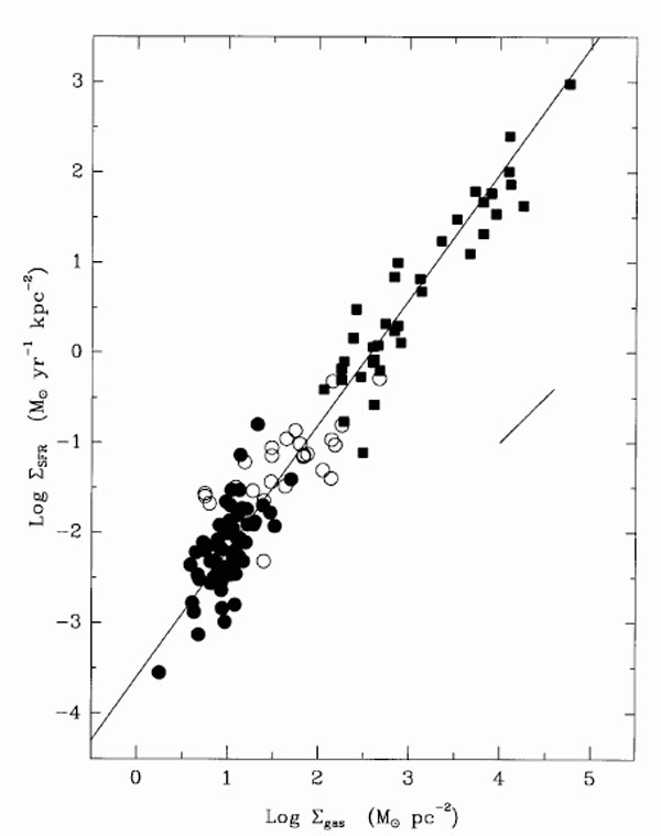 |
Figure 1. The SFR as measured by Kennicutt (1998a) in star forming galaxies. The continuous line represents the best fit to the data and it can be achieved either with the SF law in eq. (6) with k = 1.4 or with the SF law in eq. (9). The short, diagonal line shows the effect of changing the scaling radius by a factor of 2. Figure from Kennicutt (1998a). |
Other common parametrizations of the SFR include a dependence on the total surface mass density besides the surface gas density:
 |
(7) |
as suggested by observational results of Dopita & Ryder (1994) and taking into account the influence of the potential well in the star formation process (i.e. feedback between SN energy input and star formation, see also Talbot & Arnett 1975). Other suggestions concern the star formation induced by spiral density waves (Wyse & Silk 1989) with expressions like:
 |
(8) |
or
 |
(9) |
with  gas
being the angular rotation speed of gas
(Kennicutt 1998a).
Also this law provides a good fit to the data of
Figure 1.
gas
being the angular rotation speed of gas
(Kennicutt 1998a).
Also this law provides a good fit to the data of
Figure 1.
The most common parametrization of the IMF is a one-slope (Salpeter 1955) or multi-slope (Scalo 1986, 1998; Kroupa et al. 1993; Chabrier 2003) power law. The most simple example of a one-slope power law is:
 |
(10) |
generally defined in a mass range of 0.1-100
M , where
a is the normalization constant derived by imposing that
, where
a is the normalization constant derived by imposing that
 0.1100 m
 (m)
dm = 1.
(m)
dm = 1.
The Scalo and Kroupa IMFs were derived from stellar counts in the solar
vicinity and suggest a three-slope function. Unfortunately, the same
analysis cannot be done in other galaxies and we cannot test if the IMF
is the same everywhere.
Kroupa (2001)
suggested that the IMF in stellar clusters is a universal one, very
similar to the Salpeter IMF for stars with masses larger than 0.5
M. In
particular, this universal IMF is:
 |
 |
(11) |
However, Weidner & Kroupa (2005) suggested that the IMF integrated over galaxies, which controls the distribution of stellar remnants, the number of SNe and the chemical enrichment of a galaxy is generally different from the IMF in stellar clusters. This galaxial IMF is given by the integral of the stellar IMF over the embedded star cluster mass function which varies from galaxy to galaxy. Therefore, we should expect that the chemical enrichment histories of different galaxies cannot be reproduced by an unique invariant Salpeter-like IMF. In any case, this galaxial IMF is always steeper than the universal IMF in the range of massive stars.
We define the current mass distribution of local Main Sequence (MS)
stars as the present day mass function (PDMF), n(m). Let
us suppose that we know n(m) from observations.
Then, the quantity n(m) can be expressed as follows: for
stars with initial masses in the range 0.1-1.0
M which have
lifetimes larger than a Hubble time we can write:
 |
(12) |
where tG ~ 14 Gyr (the age of the Universe). The IMF,
(m),
can be taken out of the integral if assumed to be
constant in time, and the PDMF becomes:
 |
(13) |
where < >
is the average SFR in the past.
>
is the average SFR in the past.
For stars with lifetimes negligible relative to the age of the Universe,
namely for all the stars with m > 2
M, we
can write:
 |
(14) |
where  m is the
lifetime of a star of mass m.
Again, if we assume that the IMF is constant in time we can write:
m is the
lifetime of a star of mass m.
Again, if we assume that the IMF is constant in time we can write:
 |
(15) |
having assumed that the SFR did not change during the time interval between
(tG -
m) and
tG. The
quantity (tG) is the SFR at the present time.
We cannot derive the IMF betwen 1 and 2
M
because none of the previous semplifying hypotheses can be applied.
Therefore, the IMF in this mass range will depend on a quantity,
b(tG):
 |
(16) |
Scalo (1986) assumed:
 |
(17) |
in order to fit the two branches of the IMF in the solar vicinity. In Figure 2 we show the differences between a single-slope IMF and multi-slope IMFs, which are preferred according to the last studies.
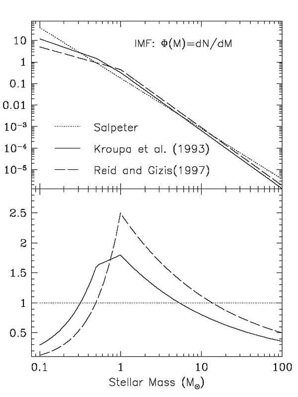 |
Figure 2. Upper panel: different IMFs. Lower panel: normalization of the multi-slope IMFs to the Salpeter IMF. Figure from Boissier & Prantzos (1999). |
The stellar yields, namely the amount of newly formed and pre-existing elements ejected by stars of all masses at their death, represent a fundamental ingredient to compute galactic chemical evolution. They can be calculated by knowing stellar evolution and nucleosynthesis.
I recall here the various stellar mass ranges and their nucleosynthesis products. In particular:
which
never ignite H. They do not enrich the interstellar medium (ISM) in
chemical elements but only lock up gas.
 M /
M
8.0).
Calculations are available from
Marigo et
al. (1996),
van den Hoeck &
Groenewegen (1997),
Forestini &
Charbonnel (1997),
Marigo (2001),
Meynet & Maeder
(2002),
Ventura et
al. (2002),
Siess et al. (2002),
Karakas &
Lattanzio (2007).
These stars produce mainly 4He,
12C, 14N plus some CNO isotopes and
s-process (A > 90) elements. In Figure 3
we show an example of integrated yields from stars in this mass range.
M /
M
8.0).
Calculations are available from
Marigo et
al. (1996),
van den Hoeck &
Groenewegen (1997),
Forestini &
Charbonnel (1997),
Marigo (2001),
Meynet & Maeder
(2002),
Ventura et
al. (2002),
Siess et al. (2002),
Karakas &
Lattanzio (2007).
These stars produce mainly 4He,
12C, 14N plus some CNO isotopes and
s-process (A > 90) elements. In Figure 3
we show an example of integrated yields from stars in this mass range.
 |
Figure 3. The yields integrated over the
Salpeter (1955)
IMF of He, C and N produced by low and intermediate mass stars
as functions of the initial stellar metallicity. Different results are
compared here: those of RV81
(Renzini & Voli
1981),
those of HG97
(van den Hoeck &
Groenewegen 1997)
and those of M2K
(Marigo 2001).
The mixing length parameters
( |
40). In the mass range 10-40
M,
available calculations are from Woosley & Weaver
(1995,
hereafter WW95),
Langer & Henkel
(1995),
Thielemann et
al. (1996),
Nomoto et
al. (1997),
Limongi & Chieffi
(2003),
Rauscher et
al. (2002),
Meynet & Maeder
(2002),
Nomoto et al. (2006),
among others. These stars end their life as Type II SNe and explode by
core-collapse; they produce mainly
 -elements
(O, Ne, Mg, Si, S, Ca), some Fe-peak elements,
s-process elements (A < 90)
and r-process elements. Stars more massive than 40
M can end up
as Type Ib/c SNe: they are also core-collapse SNe and are linked to
-elements
(O, Ne, Mg, Si, S, Ca), some Fe-peak elements,
s-process elements (A < 90)
and r-process elements. Stars more massive than 40
M can end up
as Type Ib/c SNe: they are also core-collapse SNe and are linked to
 -ray bursts
(GRB).
-ray bursts
(GRB).
).
Calculations are available from e.g.
Portinari et
al. (1998),
Umeda & Nomoto
(2001).
They should produce mainly oxygen although many uncertainties are still
present.
All the elements with mass number A from 12 to 60 have
been formed in stars during the quiescent burnings.
Stars transform H into He and then He into heaviers until the
Fe-peak elements, where the binding energy per nucleon reaches a maximum
and the nuclear fusion reactions stop.
H is transformed into He through the proton-proton chain or the
CNO-cycle, then 4He is transformed into
12C through the
triple- reaction.
Elements heavier than 12C are then produced by synthesis
of -particles: they are
called -elements
(O, Ne, Mg, Si and others).
The last main burning in stars is the 28Si -burning which produces 56Ni, which then decays into 56Co and 56Fe. Si-burning can be quiescent or explosive (depending on the temperature).
Explosive nucleosynthesis occurring during SN explosions
mainly produces Fe-peak elements. Elements
originating from s- and r-processes (with A > 60 up to Th and U)
are formed by means of slow or rapid (relative to the
 - decay)
neutron capture by Fe seed nuclei;
s-processing occurs during quiescent He-burning,
whereas r-processing occurs during SN explosions.
- decay)
neutron capture by Fe seed nuclei;
s-processing occurs during quiescent He-burning,
whereas r-processing occurs during SN explosions.
In Figures 4, 5,
6, 7 and
8 we show a comparison between stellar yields
for massive stars
computed for different initial stellar metallicities and with different
assumptions concerning the mass loss. In particular, some yields are
obtained by assuming mass loss by stellar winds with a strong dependence
on metallicity (e.g.
Maeder, 1992),
whereas others (e.g. WW95) are computed by means of conservative models
without mass loss.
One important difference arises for oxygen in massive stars for solar
metallicity and mass loss: in this case, the O yield is strongly
depressed as a consequence of mass loss. In fact, the stars with masses
> 25 M
and solar metallicity lose a large amount of matter rich of He and C,
thus subctracting these elements to further processing which would lead
to O and heavier elements. So the net effect of mass loss is to increase
the production of He and C and to depress that of oxygen (see
Figure 9). More recently,
Meynet & Mader
(2002,
2003,
2005)
have computed a grid of models for stars with M > 20
M
including rotation and metallicity dependent mass loss. The effect of
metallicity dependent mass loss in decreasing the O production in
massive stars was confirmed, although they employed significantly lower
mass loss rates compared with
Maeder (1992).
With these models they were able to reproduce the frequency of WR stars
and the observed WN/WC ratio, as was the case for the previous Maeder
results. Therefore, it appears that the earlier mass loss rates made-up
for the omission of rotation in the stellar models.
On the other hand, the dependence upon metallicities of the yields
computed with conservative stellar models, such as those of WW95, is not
very strong except perhaps for the yields computed with zero intial
stellar metallicity (Pop III stars).
 |
Figure 4. The yields of oxygen for massive stars as computed by several authors, as indicated in the Figure. None of these calculations takes into account mass loss by stellar wind. |
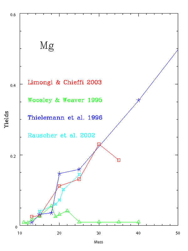 |
Figure 5. The same as Fig. 4 for magnesium. |
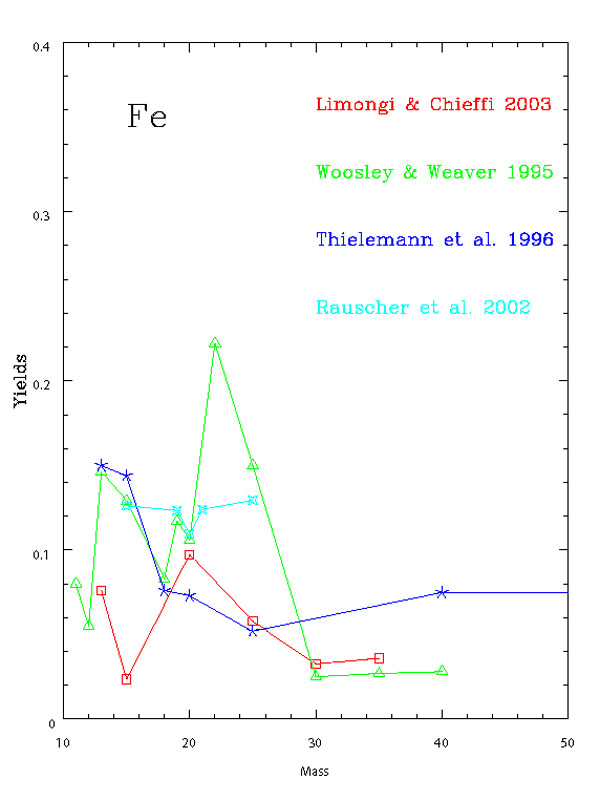 |
Figure 6. The same as Fig. 4 for Fe. |
In Figures 7 and 8 we show the most recent results of Nomoto et al. (2006) for conservative stellar models of massive stars at different metallicities. While the O yields are not much dependent upon the initial stellar metallicity, as in WW95 , the Fe yields seem to change dramatically with the stellar metallicity.
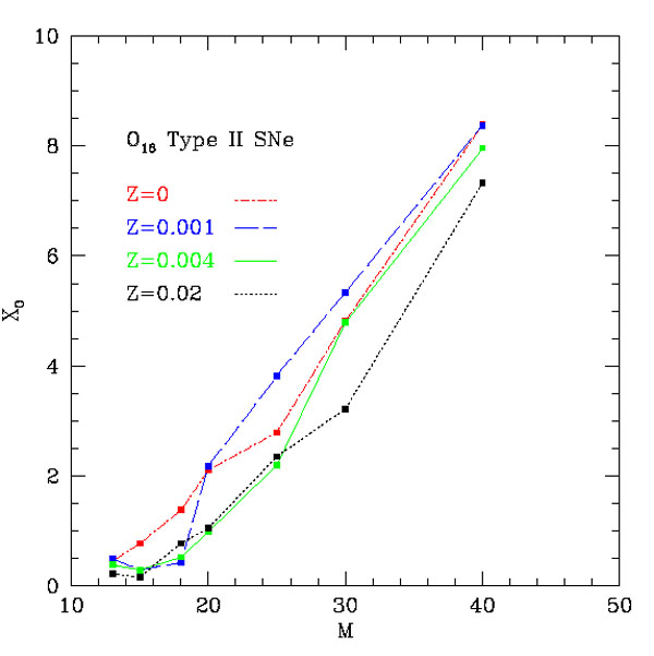 |
Figure 7. The O yields as calculated by Nomoto et al. (2006) for different metallicities. These calculations do not take into account mass loss by stellar wind. |
 |
Figure 8. The same as Figure 7 for Fe. |
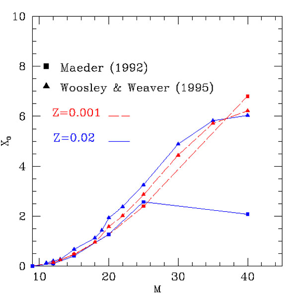 |
Figure 9. The effect of metallicity dependent mass loss on the oxygen yield. The comparison is between the conservative yields of WW95 for Z = 0.001 and Z = 0.02 and the yields with mass loss of Maeder (1992) for the same metallicity. As one can see the effect of mass loss for a solar metallicity is a quite important one. |
There is a general consensus about the fact that SNeIa originate from
C-deflagration in C-O white dwarfs (WD) in binary systems, but several
evolutionary paths can lead to such an event. The C-deflagration
produces ~ 0.6-0.7
M of Fe
plus traces of other elements from C to Si, as observed in the spectra
of Type Ia SNe.
Two main evolutionary scenarios for the progenitors of Type Ia SNe have been proposed:
after
accreting material from a red giant
companion. One of the limitations of this scenario is that the accretion
rate should be defined in a quite narrow range of values. To avoid this
problem,
Kobayashi et
al. (1998)
had proposed a similar scenario, based on the model of
Hachisu et al. (1996),
where the companion can be either a red giant or a main sequence star,
including
a metallicity effect which suggests that no Type Ia systems can form
for [Fe/H] < -1.0 dex. This is due to the development of a strong
radiative wind from the C-O WD which stabilizes the accretion from the
companion, allowing for larger mass accretion rates than the previous
scenario. The clock to the explosion is given by the lifetime of the
secondary star in the binary system, where the WD is the primary (the
originally more massive one). Therefore, the largest mass for a
secondary is 8
M, which
is the maximum mass for the formation of a C-O WD. As a consequence, the
minimum timescale for the occurrence of Type Ia SNe is ~ 30 Myr
(i.e. the lifetime of a
8 M)
after the beginning of star formation. Recent observations in
radio-galaxies by Mannucci et al.
(2005;
2006)
seem to confirm the existence of such prompt Type Ia SNe.
The minimum mass for the secondary is 0.8
M, which
is the star with lifetime equal to the age of the universe. Stars with
masses below this limit are obviously not considered.
In summary, the mass range for both primary and secondary stars is, in
principle, between 0.8 and
8M,
although two stars of 0.8
M are
too small to give rise to a WD with a Chandrasekhar mass, and therefore
the mass of the primary star should be assumed to be high enough to
ensure that, even after accretion from a
0.8 M
star secondary, it will reach the Chandrasekhar mass.
in
order to give rise to a Chandrasekhar mass after they merge, therefore
their progenitors should be in the range (5-8)
M. The
clock to the explosion here is given by the lifetime of the secondary
star plus the gravitational time delay which depends on the original
separation of the two WDs. The minimum timescale for the appearance of
the first Type Ia SNe in this scenario is a few million years more than
in the SD scenario (e.g. ~ 40 Myr in
Tornambé &
Matteucci 1986).
At the same time, the maximum gravitational time delay can be as long as
more than a Hubble time. For more recent results on the DD scenario see
Greggio (2005).
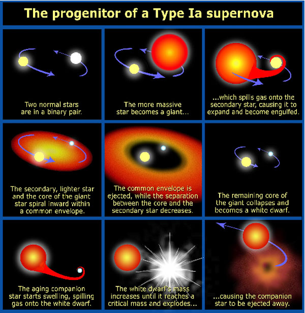 |
Figure 10. The progenitor of a Type Ia SN in the context of the single-degenerate model (Illustration credit: NASA, ESA, and A. Field (STSci)). |
Within any scenario the explosion can occur either when the C-O WD reaches the Chandrasekhar mass and carbon deflagrates at the center or when a massive enough helium layer is accumulated on top of the C-O WD. In this last case there is He-detonation which induces an off-center carbon deflagration before the Chandrasekhar mass is reached (sub-chandra exploders, e.g. Woosley & Weaver 1994).
While the chandra-exploders are supposed to produce the same nucleosynthesis (C-deflagration of a Chandrasekhar mass), they predict a different evolution of the Type Ia SN rate and different typical timescales for the SNe Ia enrichment. A way of defining the typical Type Ia SN timescale is to assume it as the time when the maximum in the Type Ia SN rate is reached (Matteucci & Recchi, 2001). This timescale varies according to the chosen progenitor model and to the assumed star formation history, which varies from galaxy to galaxy. For the solar vicinity, this timescale is at least 1 Gyr, if the SD scenario is assumed, whereas for elliptical galaxies, where the stars formed much more quickly, this timescale is only 0.5 Gyr (Matteucci & Greggio, 1986; Matteucci & Recchi 2001).
Various parametrizations have been suggested for gas flows and the most common is an exponential law for the gas infall rate:
 |
(18) |
with the timescale being a
free parameter, whereas for the galactic outflows the wind rate is
generally assumed to be proportional to the SFR:
 |
(19) |
where  is again a free
parameter. Both and
should
be fixed by reproducing the majority of observational constraints.
is again a free
parameter. Both and
should
be fixed by reproducing the majority of observational constraints.