


We will first analyze the chemical evolution of our Galaxy, the Milky Way.
3.1. The formation of the Milky Way
The Milky Way galaxy has four main stellar populations: 1) the halo stars with low metallicities 1 and eccentric orbits, 2) the bulge population with a large range of metallicities and dominated by random motions, 3) the thin disk stars with an average metallicity <[Fe / H]> = -0.5 dex and circular orbits, and finally 4) the thick disk stars which possess chemical and kinematical properties intermediate between those of the halo and those of the thin disk. The halo stars have average metallicities of <[Fe / H]> = -1.5 dex and a maximum metallicity of ~ -1.0 dex, although stars with [Fe/H] as high as -0.6 dex and halo kinematics are observed. The average metallicity of thin disk stars is ~ -0.6 dex, whereas the one of bulge stars is ~ -0.2 dex.
The kinematical and chemical properties of the different Galactic stellar populations can be interpreted in terms of the Galaxy formation mechanism. Eggen, Lynden-Bell & Sandage (1962), in a cornerstone paper suggested a rapid monolithic collapse for the formation of the Galaxy lasting ~ 2 × 10⁸ years. This suggestion was based on a kinematical and chemical study of solar neighbourhood stars and the value of the suggested timescale was chosen to allow for the orbital eccentricities to vary in a potential not yet in equilibrium but sufficiently long so that massive stars forming in the collapsing gas could have time to die and enrich the gas with heavy elements.
Later on, Searle & Zinn (1978) measured Fe abundances and horizontal branch morphologies of 50 globular clusters and studied their properties as a function of the galactocentric distance. As a result of this, they proposed a central collapse like the one envisaged by Eggen et al., but also that the outer halo formed by merging of large fragments taking place over a considerable timescale > 1 Gyr. The Searle & Zinn scenario is close to what is predicted by modern cosmological theories of galaxy formation. In particular, in the framework of the hierarchical galaxy formation scenario, galaxies form by accretion of smaller building blocks (e.g. White & Rees, 1978, Navarro & al. 1997). Obvious candidates for these building blocks are either dwarf spheroidal (dSph) or dwarf irregular (dIrr) galaxies. However, as we will see in detail later, the chemical composition and in particular the chemical abundance patterns in dSphs or dIrrs are not compatible with the same abundance patterns in the Milky Way (see Geisler et al. 2007), thus arguing against the identification of the building blocks with these galaxies. On the other hand, very recently, Carollo & al. (2007) have obtained medium resolution spectroscopy of 20,336 stars from the Sloan Digital Sky Survey (SDSS). They showed that the Galactic halo is divisible into two broadly overlapping structural components. In particular, they find that the inner halo is dominated by stars with very eccentric orbits, exhibits a peak at [Fe/H] = -1.6 dex and has a flattened density distribution with a modest net prograde rotation. The outer halo includes stars with a wide range of eccentricities, exhibits a peak at [Fe/H] = -2.2 dex and a spherical density distribution with highly statistically significant net retrograde rotation. They conclude that most of the Galactic halo should have formed by accrection of multiple distinct sub-systems. However, an analysis of the abundance ratios of these stars is still missing.
From an historical point of view, the modelization of the Galactic chemical evolution has passed through different phases that I summarize in the following:
SERIAL FORMATION
The Galaxy is modeled by means of one accretion episode lasting for the
entire Galactic lifetime, where halo, thick and thin disk form in
sequence as a continuous process. The obvious limit of this approach
is that it does not allow us to predict the observed overlapping in
metallicity between halo and thick disk stars and between thick and thin
disk stars, but it gives a fair representation of our Galaxy (e.g.
Matteucci &
François 1989).
PARALLEL FORMATION
In this formulation, the various Galactic components start at the same time
and from the same gas but evolve at different rates (e.g.
Pardi et al. 1995).
It predicts overlapping of stars belonging to the different components
but implies that the thick disk formed out of gas shed by the halo and
that the thin disk formed out of gas shed by the thick disk, and this is
at variance with the distribution of the stellar angular momentum per
unit mass
(Wyse & Gilmore
1992),
which indicates that the disk did not form out of gas shed by the halo.
TWO-INFALL FORMATION
In this scenario, halo and disk
formed out of two separate infall episodes (overlapping in metallicity
is also predicted) (e.g.
Chiappini et
al. 1997;
Chang et al. 1999;
Alibés et
al. 2001).
The first infall episode lasted no more than 1-2 Gyr whereas the second,
where the thin disk formed,
lasted much longer with a timescale for the formation of the solar
vicinity of 6-8 Gyr
(Chiappini et
al. 1997;
Boissier &
Prantzos 1999).
STOCHASTIC APPROACH
Here the hypothesis is that in the early halo phases ([Fe/H] < -3.0
dex), mixing was not
efficient and, as a consequence, one should observe, in low metallicity
halo stars, the effects of pollution from single SNe (e.g.
Tsujimoto et
al. 1999;
Argast et al. 2000;
Oey 2000).
These models predict a large spread for [Fe/H] < -3.0 dex for all the
 -elements,
which is not observed, as shown
by stellar data with metallicities down to -4.0 dex
(Cayrel et
al. 2004).
However, inhomogeneities could explain
the observed spread of s- and r-elements at low metallicities (see later).
-elements,
which is not observed, as shown
by stellar data with metallicities down to -4.0 dex
(Cayrel et
al. 2004).
However, inhomogeneities could explain
the observed spread of s- and r-elements at low metallicities (see later).
The two-infall model of
Chiappini, Matteucci
& Gratton (1997)
predicts two main episodes of gas accretion: during the first one, the
halo the bulge and most of the thick disk formed, while the second gave
rise to the thin disk.
In Figure 13 we show an artistic representation
of the formation of the Milky Way in the two-infall scenario. In the
upper panel we see the sequence of the formation of the stellar halo, in
particular the inner halo, following a monolithic-like collapse of gas
(first infall episode) but with a longer timescale than originally
suggested by
Eggen et al. (1962):
here the time scale is 0.8-1.0 Gyr. During the halo formation also the
bulge is formed on a very short timescale in the range 0.1-0.5
Gyr. During this phase also the thick disk assembles or at least part of
it, since part of the thick disk, like the outer halo, could have been
accreted. The second panel from left to right shows the beginning of the
thin disk formation, namely the assembly of the innermost disk regions
just around the bulge; this is due to the second infall episode. The
thin-disk assembles inside-out, in the sense that the outermost regions
take a much longer time to form. This is shown in the third panel. In
Fig. 13 each panel is connected to temporal
phases where the Type II and
then the Type Ia SN rates are present. So, it is clear that the early
phases of the halo and bulge formation are dominated by Type II SNe (and
also by Type Ib/c SNe) producing mostly
-elements such as O and
Mg and part of Fe. On the other hand, Type Ia SNe start to be non
negligible only after 1Gyr and they pollute the gas during the thick and
thin disk phases. The minimum shown in the Type II SN rate is due to a
gap in the star formation rate occurring as a consequence of the
adoption of a threshold density in the star formation process, as we
will see next (Figure 14).
 |
Figure 12. Schematic edge-on view of the major components of the Milky Way. Illustration credit from R. Buser, www.astro.unibas.ch/forschung/rb/structure.shtml. |
 |
Figure 13. Artistic view of the two-infall
model by
Chiappini et
al. (1997).
The predicted SN II and Ia rates per century are also sketched,
together with the fact that Type II SNe produce mostly
|
3.3. Detailed recipes for the two-infall model
The main assumption of this model are:
 .
.
 |
(33) |
where A(r, t) = (d
 (r,
t) / dt)infall is the rate at which the total
surface mass density changes because of the infalling gas. The
quantities a(r) and b(r) are two parameters
fixed by reproducing the total present time surface mass density in the
solar vicinity
(tot = 51
± 6 M
pc-2, see
Boissier &
Prantzos 1999),
tmax = 1 Gyr is the time for the maximum infall on the
thin disk,
(r,
t) / dt)infall is the rate at which the total
surface mass density changes because of the infalling gas. The
quantities a(r) and b(r) are two parameters
fixed by reproducing the total present time surface mass density in the
solar vicinity
(tot = 51
± 6 M
pc-2, see
Boissier &
Prantzos 1999),
tmax = 1 Gyr is the time for the maximum infall on the
thin disk,  H =
0.8 Gyr
is the time scale for the formation of the halo thick-disk (which means
a total duration of 2 Gyr for the complete halo-thick disk formation)
and D(r)
is the timescale for the formation of the thin disk and it is a function of
the galactocentric distance (formation inside-out,
Matteucci &
François 1989;
Chiappini et
al. 2001).
H =
0.8 Gyr
is the time scale for the formation of the halo thick-disk (which means
a total duration of 2 Gyr for the complete halo-thick disk formation)
and D(r)
is the timescale for the formation of the thin disk and it is a function of
the galactocentric distance (formation inside-out,
Matteucci &
François 1989;
Chiappini et
al. 2001).
In particular, it is assumed that:
 |
(34) |
where r is the galocentric distance.
 |
(35) |
where the constant  is the
efficiency of the SF process, as defined
in eq. (6), and is expressed in Gyr-1: in particular,
= 2 Gyr-1 for the
the halo and 1 Gyr-1 for the disk (t
is the
efficiency of the SF process, as defined
in eq. (6), and is expressed in Gyr-1: in particular,
= 2 Gyr-1 for the
the halo and 1 Gyr-1 for the disk (t
 1 Gyr).
The total surface mass density is represented by
(r, t),
whereas
(r,
t) is the total surface mass density at the solar position,
assumed to be
r = 8 Kpc
(Reid 1993).
The quantity
gas(r,
t) represents the surface gas density. The exponent of the
surface gas density, k, is set equal to 1.5, similar to what
suggested by
Kennicutt (1998a).
These choices for the parameters allow the model to fit very well the
observational constraints, in particular in the solar vicinity.
We recall that below a critical threshold for the surface gas density
(7M
pc-2 for the thin disk and
4M
pc-2 for the halo phase)
we assume that the star formation is halted. The existence of a
threshold for the star formation has been suggested by
Kennicutt (1998a,
b)
and
Martin & Kennicutt (2001).
1 Gyr).
The total surface mass density is represented by
(r, t),
whereas
(r,
t) is the total surface mass density at the solar position,
assumed to be
r = 8 Kpc
(Reid 1993).
The quantity
gas(r,
t) represents the surface gas density. The exponent of the
surface gas density, k, is set equal to 1.5, similar to what
suggested by
Kennicutt (1998a).
These choices for the parameters allow the model to fit very well the
observational constraints, in particular in the solar vicinity.
We recall that below a critical threshold for the surface gas density
(7M
pc-2 for the thin disk and
4M
pc-2 for the halo phase)
we assume that the star formation is halted. The existence of a
threshold for the star formation has been suggested by
Kennicutt (1998a,
b)
and
Martin & Kennicutt (2001).
The predicted behaviour of the SFR, obtained by adopting eq.(35) with the threshold is shown in Figure 14.
 |
Figure 14. The SFR in the solar vicinity as predicted by the two-infall model. Figure from Chiappini et al. (1997). The oscillating behaviour in the SFR at late times is due to the assumed threshold density for SF. The threshold gas density is also responsible for the gap in the SFR seen at around 1 Gyr. |
 |
Figure 15. The Type II and Ia rate in the solar vicinity as predicted by the two-infall model. Figure from Chiappini et al. (1997). The oscillating behaviour of the Type II SN rate at late times is due to the assumed threshold density for SF. The threshold gas density is also responsible for the gap in the SFR seen at around 1 Gyr. |
3.4. The chemical enrichment history of the solar vicinity
We study first the solar vicinity, namely the local ring at 8 Kpc from
the galactic center. By integrating eq. (32) without the wind term we
obtain the evolution of the abundances of several
chemical species (H, D, He, Li, C, N, O,
-elements,
Fe, Fe-peak elements, s-and r- process elements).
In Figure 16 we show the smallest mass dying at
any cosmic time corresponding to a given predicted abundance of [Fe/H]
in the ISM. This is because there is an age-metallicity relation and the
[Fe/H] abundance increases with time. We recall that, for a generic
chemical element i, with abundance Xi, one
defines:
 |
(36) |
where log(Xi /
H)
refers to the solar abundance of the element i.
A good model of chemical evolution should be able to reproduce a minimum
number of observational constraints and the number of observational
constraints should be larger than the number of free parameters which
are: H,
D,
k1, k2,
and A (the
fraction of binary systems which can give rise to Type Ia SNe).
The main observational constraints in the solar vicinity that a good model should reproduce (see Chiappini et al. 2001, Boissier & Prantzos, 1999 and references therein) are:
gas = 13 ± 3
M
pc-2
* =
43 ± 5
M
pc-2
tot = 51 ± 6
M
pc-2
 o
= 2-5 M
pc-2 Gyr-1
o
= 2-5 M
pc-2 Gyr-1
pc-2 Gyr-1
And finally, a good model of chemical evolution of the Milky Way should reproduce the distributions of abundances, gas and star formation rate along the disk as well as the average observed SNII and Ia rates (SNII = 1.2 ± 0.8 × 100 yr-1 and SNIa = 0.3 ± 0.2 × 100 yr-1).
 |
Figure 16. In this figure we show the smallest stellar mass which dies at any given [Fe/H] achieved by the ISM as a consequence of chemical evolution. Thus, it is clear that in the early phases of the halo only massive stars are dying and contributing to the chemical enrichment process. Clearly this graph depends upon the assumed stellar lifetimes and upon the age-[Fe/H] relation. It is worth noting that the Fe production from Type Ia SNe appears before the gas has reached [Fe/H] = 1.0, therefore during the halo and thick disk phase. This clearly depends upon the assumed Type Ia SN progenitors (in this case the single degenerate model). |
What we call time-delay model is the interpretation of the behaviour of
abundance ratios such
[/Fe] (where
-elements are O, Mg, Ne,
Si, S, Ca and Ti) versus [Fe/H], a typical way of plotting the
abundances measured in the stars. The time-delay refers to the delay
with which Fe is ejected into the ISM by SNe Ia relative to the fast
production of
-elements by
core-collapse SNe.
Tinsley (1979)
first suggested that this time delay would have produced a typical
signature in the [/Fe]
vs. [Fe/H] diagram. In the following years,
Greggio & Renzini
(1983b),
by means of simple models (star formation burst or constant star
formation) studied the effects of the delayed Fe production by Type Ia
SNe on the [O/Fe] vs. [Fe/H] diagram.
Matteucci &
Greggio (1986)
included for the first time the Type Ia SN rate formulated by
Greggio & Renzini
(1983a)
in a detailed numerical model for the chemical
evolution of the Milky Way. The effect of the delayed Fe production is
to create an overabundance
of O relative to Fe ([O/Fe] > 0) at low [Fe/H] values, and a
continuous decline of the [O/Fe] ratio until the solar value
([O/Fe] = 0.0)
is reached for [Fe/H] > -1.0 dex. This is what is observed and
indicates that during the halo phase the [O/Fe] ratio is due only to the
production of O and Fe by SNe II. However, since the bulk of Fe is
produced by Type Ia SNe, when these latter start to be important then
the [O/Fe] ratio begins to decline. This effect was predicted by
Matteucci &
Greggio (1986)
to occur also for other
-elements (e.g. Mg,
Si). At the present time, a great amount of stellar abundances is
available and the trend of the
-elements has been
confirmed. Before showing some of the most recent data, it is worth
showing better the time-delay model.
In Figure 17 it is shown that a good fit of the
[O/Fe] ratio as a function of [Fe/H] is obtained only if the
-elements are mainly
produced by Type II SNe and the Fe by Type Ia SNe. If one assumes that
only SNe Ia produce Fe as well as if one assumes that only Type II SNe
produce Fe, the agreement with observations is lost. Therefore, the
conclusion is that both Types of SNe should produce Fe in the
proportions of 1/3 for Type II SNe and 2/3 for Type Ia SNe. The
IMF also plays a role in this game and these proportions are obtained
for "normal" Salpeter-like IMFs, which includes both
Salpeter (1955) and
Scalo (1986) or
Kroupa et al. (1993)
IMFs.
 |
Figure 17. The relation between [O/Fe] vs. [Fe/H] for Galactic stars in the solar vicinity. The models and the data are normalized to the solar meteoritic abundances of Anders & Grevesse (1989). The thick curve represents the predictions of the two-infall model where Type Ia SNe produce ~ 70% of Fe and Type II SNe the remaining ~ 30%. The upper thin curve represents the case where all the Fe is assumed to be produced by Type Ia SNe, whereas the thin lower line refers to the case where all the Fe is assumed to be produced in Type II SNe. The data are from Melendez & Barbuy (2002). |
As a further illustration of the time-delay model we show in Figures 18, 19 and 20 the [Xi/Fe] vs. [Fe/H] relations both observed and predicted for stars in the solar vicinity belonging to halo, thick- and thin-disk. The adopted yields for massive stars are those suggested by François et al. (2004) in order to best fit these relations and the solar abundances (namely the abundances in the ISM 4.5 Gyr ago). These yields are obtained by applying some corrections to the yields of WW95, as shown in Figure 21, where the ratios between the suggested and WW95 yields are reported.
 |
Figure 18. Predicted and observed
[ |
 |
Figure 19. The same as Fig. 18 for Ni, Zn, K and Sc. The models and the data are from François et al. (2004). The models are normalized to the predicted solar abundances. The predicted abundance ratios at the time of the Sun formation are shown in each panel and indicate a good fit. |
 |
Figure 20. The same as in Fig. 18 for Ti, Cr, Mn and Co. The models and the data are from François et al. (2004). The models are normalized to the predicted solar abundances. The predicted abundance ratios at the time of the Sun formation are shown in each panel and indicate a good fit. |
 |
Figure 21. Ratios between the empirical yields derived by François et al. (2004) and the yields of WW95 for massive stars. In the small panel at the bottom right we show the same ratios for SNe Ia and the comparison is with the yields of Iwamoto et al. (1999). |
In Figure 22 we show the predictions of a chemical evolution model for the solar vicinity where the recent yields from massive stars of Nomoto et al. (2006) have been adopted. As one can see, although some of the problems present in the previous yields have been alleviated, for other elements the disagreement still persists.
 |
Figure 22. Predicted and observed [X/Fe] vs. [Fe/H] in the solar neighbourhood. The predictions are from Nomoto et al. (2006), where all the references to the data can be found, and they have been obtained by means of metal dependent yields. Figure from Nomoto et al. (2006). |
The G-dwarf metallicity distribution and constraints on the thin disk formation
The G-dwarf metallicity distribution is a quite important constraint for the chemical evolution of the solar vicinity. It is the fossil record of the star formation history of the thin disk. If one is able to reproduce such a distribution, then one can have an idea of the SFR and the IMF and, as a consequence, of the gas accretion history. Therefore, to fit the G-dwarf metallicity distribution means to obtain constraints on the mechanism of formation of the thin disk. Originally, there was the "G-dwarf problem" which means that the Simple Model of galactic chemical evolution could not reproduce the distribution of the G-dwarfs. It has been since long demonstrated that relaxing the closed-box assumption and allowing for the solar region to form gradually by accretion of gas can solve the problem (Tinsley, 1980; Pagel 1997). Also a variable IMF could solve the problem but it would create other problems (see Martinelli & Matteucci, 2000). Assuming that the disk forms from pre-enriched gas can also solve the problem but still the gas infall is necessary to have a realistic picture of the disk formation. The two-infall model can reproduce very well the G-dwarf distribution and also that of K-dwarfs (see Figures 23 and 24), as long as a timescale for the formation of the disk in the solar vicinity of 7-8 Gyr is assumed. This conclusion is shared by other authors (Alibés et al. 2001; Prantzos & Boissier 1999)
 |
Figure 23. The G-dwarf metallicity distribution. The model prediction is from Chiappini et al. (1997) and assumes a timescale for the formation of the local disk of 8 Gyr. The data are represented by the histograms. |
 |
Figure 24. The figure is from
Kotoneva et al. (2002)
and shows the comparison between a sample of K-dwarfs and model
predictions in the solar neighbourhood. The dotted curve refers to the
two-infall model with a timescale
|
Carbon and nitrogen deserve a separate discussion from the other elements, in particular 14N whose observational behaviour is difficult to reconcile with the theory. First of all, we should distinguish between primary and secondary elements: primary elements are those synthesized directly from H and He, whereas secondary elements are those deriving from metals already present in the star at birth. In the framework of the Simple Model of galactic chemical evolution, the abundance of a secondary element evolves like the square of the abundance of the progenitor metal, whereas the evolution of the abundance of a primary element does not depend on the metallicity.
In Figure 25 we show the predictions of the
Simple Model for the ratio N/O, together with data for extragalactic HII
regions and Damped
Lyman- systems (DLAs).
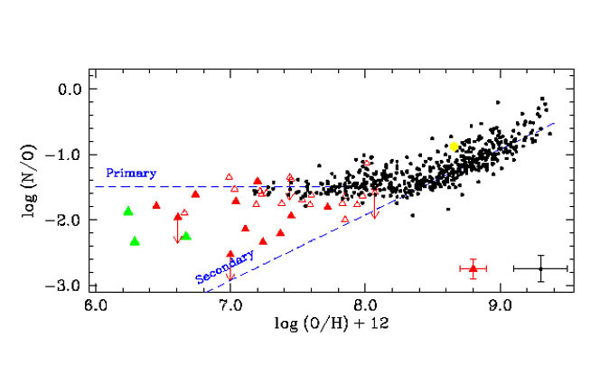 |
Figure 25. The plot of log (N/O)
vs. log(O/H) + 12: small dots represent extragalactic HII regions, red
triangles are Damped-Lyman
|
It is worth noting that the solutions of the Simple Model for a primary and a secondary element are oversemplifications since the Simple Model does not take into account stellar lifetimes which are very important in 14N production, which arises mainly from low and intermediate mass stars, both as a secondary and primary element (e.g. Renzini & Voli, 1981; van den Hoeck & Groenewegen 1997). Also 12C originates mainly from low and intermediate mass stars. The contribution to 12C from massive stars becomes very important only for metallicities oversolar, if the metallicity dependent mass loss is adopted (e.g. Maeder 1992).
The interpretation of the diagram of Figure 25 is not so straightforward since extragalactic HII regions and DLAs are galaxies, and not necessarily that diagram is an evolutionary one, in the sense that O/H does not trace the time unlike [Fe/H] in the Galactic stars. Galaxies, in fact, may have started forming stars at different cosmic epochs and with different SF histories. However, if we interpret the diagram of Figure 25 as an evolutionary one, then the DLAs and the extragalactic HII regions of low metallicity should be younger and reflect the nucleosynthesis in massive stars and perhaps in intermediate mass stars. The observed plateau for N/O at low metallicity then would indicate a primary production of N in massive stars. Nitrogen, in fact, is also produced in massive stars: until a few years ago, the N production in massive stars was considered only a secondary process, until Meynet & Maeder (2002, 2003, 2005) showed that stellar rotation in massive stars can produce primary N. A better test for the primary/secondary nature of N is represented by the Galactic stars, since they really represent an evolutionary sequence. In Figures 26 and 27 we show the most recent data on C and N compared with chemical evolution models including N from rotating massive stars.
 |
Figure 26. Upper panel: solar vicinity diagram log(N/O) vs. log(O/H) + 12. The data points are from Israelian et al. (2004) (large squares) and Spite et al. (2005) (asterisks). Models: the dashed line represents a model with substantial primary N production from massive stars. This was obtained by means of stellar models (Meynet et al. 2006; Hirschi 2007) with faster rotation relative to the work of Meynet & Maeder (2002) for Z = 10-8. Lower panel: solar vicinity diagram log(C/O) vs. log(O/H) + 12. The data are from Spite et al. (2005) (asterisks), Israelian et al. (2004) (squares) and Nissen (2004) (filled pentagons). Solar abundances (Asplund et al. 2005, and references therein) are also shown. Figure from Chiappini et al. (2006). |
As one can see in Figures 26 and 27, the fit with data is good when primary N from massive stars is included. However, there are a few warnings, first of all the measurements of N abundance in stars of low metallicity are still uncertain and then the fact that the N measurement in the gas in DLAs at high redshift show that at low O abundances there are systems with a log(N/O) < -2.0, below the plateau shown by Galactic stars. A plateau in [N/Fe]is also observed in Galactic stars for [Fe/H] < -3.0 dex, as shown in Figure 27. In Figure 27 we show also the [C/Fe] values for Galactic stars but only for low metallicity stars: they indicate a roughly solar ratio like the stars with higher metallicities. Therefore, both [N/Fe] and [C/Fe] seem to show roughly constant solar values over the total [Fe/H] range. In the framework of the time-delay model, this means that C, N and Fe are all formed in the same stars (or with the same lifetimes) and that N is mainly a primary element. However, more data are necessary to assess this point and to reconcile the Galactic star data with high redshift DLAs.
 |
Figure 27. Observed and predicted [C/Fe] vs. [Fe/H] (upper panel) and [N/Fe] vs. [Fe/H] (bottom panel) in the solar neighbourhood. The data points are from Cayrel et al. (2004), Spite et al. (2005) (asterisks) and Israelian et al. (2004) (squares). The dot-dashed line represents a model with yields from Chieffi & Limongi (2002, 2004) for a metallicity Z = 10-6 connected to the Pop III stars (only massive stars for that metallicity). The dashed line and the dotted lines represent heuristic models where the yields of C and N have been assumed "ad hoc". In particular, the fraction of primary N from massive stars is obtained by the fit to the data at low metallicity. Figure from Chiappini, Matteucci & Ballero (2005). |
The s- and r- process elements are generally
produced by neutron capture on Fe seed nuclei. The former
are formed during the He-burning phase both in low and massive stars,
whereas the latter occur in explosive events such as Type II
SNe. Recently,
François et
al. (2006)
have measured the abundances of several very heavy elements (e.g. Ba and
Eu) in extremely metal poor stars of the Milky Way. Previous work on the
subject had shown a large spread in the abundance ratios of these
elements to iron, especially at low metallicities. This spread is
confirmed by this more recent study although is less than before, and is
at variance with the lack of spread observed in the other elements shown
before (e.g.
-elements).
Apart from this problem, not yet solved, these diagrams can be very
useful to place constraints on the nucleosynthetic origin of these
elements. In particular,
Cescutti et
al. (2006)
by adopting the two-infall model predicted the evolution of [Ba/Fe] and
[Eu/Fe] versus [Fe/H], as shown in Figures 28
and 29. They can well fit the average trend but
not the spread at very low metallicities since the model assumes
instantaneous mixing. In order to fit the Ba evolution, they assumed
that Ba is mainly produced as s-process element in low mass stars (1-3
M) but
that a fraction of Ba is also produced as an r-process element in stars
with masses 12-30
M.
Europium is assumed to be only an r-process element
produced in the range 12-30
M.
 |
Figure 28. The evolution of Barium in the solar vicinity as predicted by the two-infall model (Cescutti et al. 2006). Data are from François et al. (2006). |
 |
Figure 29. The evolution of Europium in the solar vicinity (Cescutti et al. 2006). Data are from François et al. (2006). |
In order to explain why the s- and r- process elements show a large and
probably real spread at very low metallicities, whereas elements such as
the -elements show only
a little spread, one could think of a moderately inhomogeneous model
coupled with differences in the nucleosynthesis between s- and r-
process elements on one side and
-elements on the other
side (see
Cescutti 2008).
Highly inhomogeneous models for the halo evolution, in fact, predict a
too large spread for the
-elements at low
metallicity (e.g.
Argast et
al. 2000).
It is worth noting the typical secondary behaviour of Ba, whose main
production is by means of the s-process, which needs Fe seed nuclei
already present in the star, and neutrons which are accreted on these
nuclei. The production of neutrons is also dependent on the original
metal content, therefore it would be even more precise to speak of Ba as
a tertiary element.
A good model of chemical evolution for the Milky Way should reproduce also the features of the Galactic disk. In particular: abundance gradients, gas and SFR distribution with the galactocentric distance.
The chemical abundances measured along the disk of the Galaxy suggest that the metal content decreases from the innermost to the outermost regions, in other words there is a negative gradient in metals. Abundance gradients can be derived from HII regions, planetary nebulae (PNe), open clusters and stars (O,B stars and Cepheids). There are two types of abundance determinations in HII regions: one is based on recombination lines which should have a weak dependence on the temperature of the nebula (He, C, N, O), the other is based on collisionally excited lines where a strong dependence is intrinsic to the method (C, N, O, Ne, Si, S, Cl, Ar, Fe and Ni). This second method has predominated until now. A direct determination of the abundance gradients from HII regions in the Galaxy from optical lines is difficult because of extinction, so usually the abundances for distances larger than 3 Kpc from the Sun are obtained from radio and infrared emission lines.
Abundance gradients can also be derived from optical emission lines in PNe. However, the abundances of He, C and N in PNe are giving only information on the internal nucleosynthesis of the star. So, to derive gradients one should look at the abundances of O, S and Ne, unaffected by stellar processes. Abundance gradients are derived also from measuring the Fe abundance in open clusters (e.g. Carraro et al. 2004; Yong et al. 2005) or from abundances in Cepheids (e.g. Andrievsky et al. 2002a, b, c, 2004; Luck et al. 2003; Yong et al. 2006) or from abundances in O, B stars (e.g. Daflon & Cunha, 2004).
In Figure 30 we show theoretical predictions of abundance gradients along the disk of the Milky Way compared with data from HII regions, B stars and PNe. The adopted model is from Chiappini et al. (2001) and is based on an inside-out formation of the thin disk. The assumed model does not allow for exchange of gas between different regions of the disk. The disk is, in fact, divided in several concentric shells 2 Kpc wide with no interaction between them.
 |
Figure 30. Spatial and temporal behaviour of abundance gradients along the Galactic disk as predicted by the best model of Chiappini et al. (2001). The upper lines in each panel represent the present time gradient, whereas the lower ones represent the gradient a few Gyr ago. It is clear that the gradients tend to stepeen in time, a still controversial result. The data are from HII regions, B stars and PNe (see Chiappini et al. 2001). |
As already mentioned, most of the current models agree on the inside-out scenario for the disk formation, however not all models agree on the evolution of the gradients with time. In fact, some models, although assuming an inside-out formation of the disk, predict a gradient flattening with time (Boissier & Prantzos 1999; Alibès et al. 2001), whereas others such as that of Chiappini et al. (2001) predict a steepening, as shown in Figure 30. The reason for the steepening is that in the model of Chiappini et al. there is included a threshold density for SF, which induces the SF to stop when the density decreases below the threshold. This effect is particularly strong in the external regions of the Galactic disk, thus contributing to a slower evolution and therefore to a steepening of the gradients with time. In Figure 31 we show models and some more recent data including Cepheids.
 |
Figure 31. Gradients of the
|
In the Chiappini et al. model, the fit to the gradients is obtained by means of the inside-out formation of the Galactic disk. Numerical simulations of abundance gradients show that no gradient arises if one assumes the same timescale of disk formation at any galactocentric distance. The different timescale of accretion influences the SFR, thus creating a gradient in the SFR and therefore in the resulting metal content. However, it should be said that the effect of the threshold is also important and tends to steepen the gradients.
In Figure 32 we show the results of Boissier & Prantzos (1999) for abundance gradients and also for the gas and SFR distribution along the disk. Note the gradients are flattening with time.
 |
Figure 32. Comparison between model predictions and observations for the disk of the Milky Way. The figure is from Boissier & Prantzos (1999). Top left panel: gas distribution along the disk. Top right panel: the O gradient at the present time (curve with label 13.5) and at two other different cosmic epochs (5 Gyr and 1 Gyr from the beginning). Second left panel: the surface mass density of living stars. Second right panel: the Fe gradient. Third left panel: the gradient of the SFR normalized to the value at the solar ring. Third right panel: the predicted distribution of the current surface mass densities of stellar remnants (WDs), black holes (BH) and neutron stars (NS). Fourth left panel: the predicted infall rate along the disk at three different cosmic epochs. Fourth right panel: the predicted distributions of surface densities by number of the stellar remnants. |
The bulges of spiral galaxies are generally distinguished in true bulges, hosted by S0-Sb galaxies and "pseudobulges" hosted in later type galaxies (see Renzini 2006 for references). Generally, the properties (luminosity, colors, line strenghts) of true bulges are very similar to those of elliptical galaxies. In the following, we will refer only to true bulges and in particular to the bulge of the Milky Way. The bulge of the Milky Way is, in fact, the best studied bulge and several scenarios for its formation have been put forward in past years. As summarized by Wyse & Gilmore (1992) the proposed scenarios are:
In the context of chemical evolution, the Galactic bulge was first
modeled by
Matteucci &
Brocato (1990)
who predicted that the
[/Fe] ratio for some
elements (O, Si and Mg) should be
supersolar over almost the whole metallicity range, in analogy with
the halo stars, as a consequence of assuming a fast bulge evolution
which involved rapid gas enrichment in Fe mainly by Type II SNe.
At that time, no data were available for chemical abundances; the
predictions of
Matteucci &
Brocato (1990)
were confirmed for a few
-elements (Mg,
Ti) by the observations of McWilliam & Rich
(1994,
hereafter MR94), whereas
for other -elements
(e.g. Ca, Si) the observed trend was different.
Other discrepancies regarding the Mg overabundance came from
Sadler et
al. (1996).
In order to better assess these points,
Matteucci et
al. (1999)
studied a larger set of abundance ratios, by means of a detailed
chemical evolution model whose parameters were calibrated so that the
metallicity distribution observed by MR94 could be fitted.
They concluded that an evolution much faster than that in the solar
neighbourhood and even faster than that of the halo (see also Renzini,
1993) is necessary for the MR94 metallicity distribution to be
reproduced, and that an IMF index flatter (x = 1.1-1.35) than
that of the solar neighbourhood is needed as well.
They also made predictions about the evolution of several abundance
ratios which were meant to be confirmed or disproved by subsequent
observations, namely that
-elements should in
general be overabundant with respect to Fe, but some (e.g. Si, Ca) less
than others (e.g. O, Mg), and that the [12C/Fe] ratio should
be solar at all metallicities.
Samland et al. (1997) developed a self-consistent chemo-dynamical model for the evolution of the Milky Way components starting from a rotating protogalactic gas cloud in virial equilibrium, which collapses owing to dissipative cloud-cloud collisions. They found that self-regulation due to a bursting star formation and subsequent injection of energy from Type II supernovae led to the development of "contrary flows", i.e. alternate collapse and outflow episodes in the bulge. This caused a prolonged star formation episode lasting over ~ 4 × 10⁹ yr. They included stellar nucleosynthesis of O, N and Fe, but claimed that gas outflows prevent any clear correlation between local star formation rate and chemical enrichment. With their model, they could reproduce the oxygen gradient of HII regions in the equatorial plane of the Galactic disk and the metallicity distribution of K giants in the bulge (Rich, 1988), field stars in the halo and G dwarfs in the disk, but they did not make predictions about abundance ratios in the bulge. In general, hierarchical clustering models of galaxy formation do not support the conclusion of a fast formation and evolution of the bulge. In Kauffmann (1996) the bulges form through violent relaxation and destruction of disks in major mergers. The stars of the destroyed disk build the bulge, and subsequently the bulge has to be rebuilt. This implies that late type spirals should have older bulges than early type ones, since the build-up of a large disk needs a long time during which the galaxy has to evolve undisturbed. This is not confirmed by observations, since the high metallicity and the the narrow age distribution observed in bulges of local spirals are not compatible with their merger origin (see Wyse, 1999).
Mollá et
al. (2000)
proposed a multiphase model in the context of
the dissipative collapse scenario of the
Eggen et al. (1962)
picture. They supposed that the bulge formation occurred in two main
infall episodes, the first from the halo to the bulge, on a timescale
H = 0.7 Gyr, and the
second from the bulge to a so-called core population in the very
nuclear region of the Galaxy, on a timescale
B
>> H.
The three zones (halo, bulge, core) interact via supernova winds and
gas infall. They concluded that there is no need for accretion of external
material to reproduce the main properties of bulges and that the
analogy to ellipticals is not justified.
Because of their rather long timescale for the bulge formation, these
authors did not predict a noticeable difference in the trend of the
[/Fe] ratios but rather
suggested that they behave more akin to that in the solar neighbourhood
(contrary to several indications from abundance data, e.g.
MR94).
Immeli et
al. (2004)
investigated the role of cloud dissipation in the formation and
dynamical evolution of star forming gas rich disks by means of a 3D
chemodynamical model.
They found that the galaxy evolution proceeds very differently depending
on whether the gas disk or the stellar disk first become unstable. This
in turn depends on how efficiently the cold cloud medium can dissipate
energy. If the gas cools efficiently, a starburst takes place which
gives rise to enhanced
[/Fe] ratios,
thus in agreement with a fast bulge formation.
A more recent model was proposed by Costa et al. (2005), in which the best fit to observations is achieved by means of a double infall model. An initial fast (0.1 Gyr) collapse of primordial gas is followed by a supernova-driven mass loss and then by a second slower (2 Gyr) infall episode, enriched by the material ejected by the bulge during the first collapse. Costa et al. (2005) claimed that the mass loss is necessary to reproduce the abundance distribution observed in PNe, and because the predicted abundances would otherwise be higher than observed. However, it should be noted again that the abundances derived from PNe can be affected by internal stellar processes and therefore are meaningless for studying galactic chemical evolution. With their model, they are able to reproduce the trend of [O/Fe] abundance ratio observed by Pompéia et al. (2003) and the data of nitrogen versus oxygen abundance observed by Escudero & Costa (2001) and Escudero et al. (2004). It must be noted however that Pompéia et al. (2003) obtained abundances for "bulge-like" dwarf stars. This "bulge-like" population consists of old (~ 10-11 Gyr) metal-rich nearby stars whose kinematics and metallicity suggest an inner disk or bulge origin and a mechanism of radial migration, perhaps caused by the action of a Galactic bar, but the birthplace of these stars is undoubtedly not certain.
Interpretation of bulge data and other galaxies
In summary, MR94 first measured the metallicity distribution and the
[/Fe] ratios in the
Galactic bulge and confirmed partly the predictions of
Matteucci &
Brocato (1990)
that all of the -elements
should be enhanced relative to Fe for a large range of [Fe/H]. In fact,
MR94 found that not all the
-elements were enhanced,
in particular oxygen. Very recently, medium- and high-resolution
spectroscopy of bulge stars was performed
(Rich &
McWilliam, 2000;
Fulbright et al.,
2006,
2007;
Zoccali et al.,
2006;
Lecureur et
al. 2007),
and it seems to indicate that also O is enhanced, thus supporting the
suggestion of a fast formation of the bulge.
The metallicity distribution of stars in the bulge and the
[/Fe] ratios
greatly help in selecting the most probable scenario for the bulge
formation. In Figure 33 we present the
predictions by
Matteucci (2003)
of the [/Fe] ratios as
functions of [Fe/H] in galaxies of different morphological type. In
particular, for the Galactic bulge or an elliptical galaxy of the same
mass, for the solar vicinity region and for an irregular magellanic
galaxy (LMC and SMC).
The underlying assumption is that different objects undergo different
histories of star formation, being very fast in the spheroids (bulges
and ellipticals), moderate in spiral disks and slow and perhaps gasping
in irregular gas rich galaxies. The effect of different star formation
histories is evident in Figure 33 where the
predicted [/Fe] ratios
in the bulge and ellipticals remain high and almost constant for a large
interval of [Fe/H]. This is due to the fact that, since star formation
is very intense, the bulge reaches very soon a solar metallicity thanks
only to the SNe II; then, when SNe Ia start exploding and ejecting Fe
into the ISM,
the change in the slope occurs at larger [Fe/H] than in the solar vicinity.
In the extreme case of irregular galaxies the situation is opposite:
here the star formation is slow and when the SNe Ia start exploding the
gas is still very metal poor.
This scheme is quite useful since it can be used to identify galaxies
only by looking at their abundance ratios. A model for the bulge
behaving as shown in Figure 33 is able to
reproduce also the observed metallicity distribution of bulge stars (see
Matteucci &
Brocato 1990;
Matteucci et
al. 1999).
The scenario suggested in these papers
favors the formation of the bulge by means of a short and strong
starburst, in agreement with
Elmegreen (1999)
and
Ferreras et
al. (2003).
A similar model, although updated with the inclusion of the development
of a galactic wind and more recent stellar yields, has been presented by
Ballero et
al. (2007):
it shows how a model with intense star formation (star formation
efficiency ~ 20 Gyr-1) and rapid assembly of gas (0.1 Gyr)
can best reproduce the most recent accurate data on abundance ratios and
metallicity distribution.
 |
Figure 33. The predicted
[ |
In Figures 34 and 35 we show a detailed comparison between model predictions for the Galactic bulge and data on O and Mg.
 |
Figure 34. The predicted [O/Fe] vs. [Fe/H] relation for the Bulge (curve), compared with the most recent data. The chemical evolution model is that of Ballero et al. (2007), where references to the data can be found. |
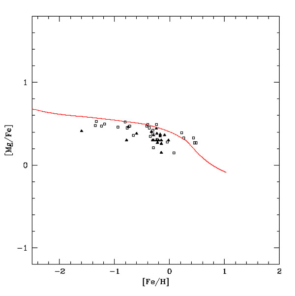 |
Figure 35. The predicted [Mg/Fe] vs. [Fe/H] relation for the bulge (curve), compared with the most recent data. The chemical evolution model is that of Ballero et al. (2007), where references to the data can be found. |
As one can see, the plateau in the
[/Fe] is longer than in
the solar neighbourhood, since in the bulge the slope of the
[/Fe] ratio starts
changing drastically only for [Fe/H] > 0.0 dex. The long plateau is
well explained by the model of
Ballero et
al. (2007)
assuming a very fast formation of the bulge. It is worth noting that the
[O/Fe] ratio has a steeper slope than [Mg/Fe] and this could be due to
differences in the nucleosynthesis of these elements (e.g.
McWilliam et
al. 2007).
The IMF assumed for the bulge is usually flatter than the IMF of the solar neighbourhood and this is generally dictated by the fit of the bulge metallicity distribution which peaks at a higher [Fe/H] than the G-dwarf metallicity distribution in the solar vicinity. Numerical calculations have indicated that the main parameter influencing the peak of the distribution is the IMF, as clearly shown in Figures 36 and 37.
 |
Figure 36. The predicted and observed
metallicity distribution in the Galactic bulge. The data are from
Zoccali et
al. (2003)
(dashed histogram) and
Fulbright et
al. (2006)
(continuous histogram). In particular, the model with the peak at the
lower metallicity is computed with an IMF which is similar to that of
the solar vicinity and indicated by IGIMF, whereas the distribution
which best fits the data is computed with a flat IMF (x = 0.95 for
M > 1
M |
 |
Figure 37. The predicted and observed metallicity distribution in the Galactic bulge. The data are from Zoccali et al (2003) (dashed histogram) and Fulbright et al. (2006) (continuous histogram). The lines are the predictions of models with the same IMF but different SF efficiencies, as indicated in the Figure. |
In summary, the comparison between the models
(Ballero et
al. 2007)
on one side, and the metallicity distribution and the
[/Fe] ratios on the
other, strongly indicates that the Galactic bulge is very old and must
have formed very quickly during a strong starburst (with a SF efficiency
much higher than in the disk). The metallicity distribution in
particular, seems to suggest an IMF flatter than in the disk
with an exponent for massive stars in the range x =
1.35-0.95. However, to assess more precisely
this point we need more data: in particular, a flatter IMF predicts that
the overabundances of
-elements relative to Fe
and to the Sun should be higher in the bulge than in the disk. This is
not entirely clear from the available data, although
Zoccali et
al. (2006)
conclude that the [O/Fe] ratios in bulge stars are higher than in thick
and thin disk stars (see Figure 38). The
timescale for the bulge formation by accretion of gas lost from the halo
is 0.1 Gyr and certainly no longer than 0.5 Gyr.
 |
Figure 38. Upper panel: the [O/Fe] vs. [Fe/H] for bulge stars as measured by Zoccali et al. (2006) (circles), along with previous determinations in other bulge stars from optical (open triangles) and near-IR spectra (crosses). Open symbols refer to spectra with lower S/N or with the O line partially blended with telluric absorption. Lower panel: [O/Fe] trend in the bulge and in thick and thin disk stars (crosses and triangles). The solid line shows a linear fit to the thick data points with [Fe/H] > -0.5 dex and is meant to emphasize that all bulge stars with -0.4 < [Fe/H] < +0.1 are more O-enhanced than the thick disk stars. If confirmed, this trend may indicate a flatter IMF for the bulge than for the disk. This plot also suggests that there is a systematic difference between bulge and disk stars, thus excluding that bulge stars were once disk stars migrated in the bulge. Figure and references from Zoccali et al. (2006). |
1 the most common
stellar metallicity indicator in stars is [Fe/H] = log(Fe /
H)* - log(Fe /
H)
Back.