


In this section, we will review the globular cluster luminosity function (GCLF) as a distance indicator. The method is currently "unfashionable" in the literature mainly because some previous results seem to be in contradiction with other distance indicators (e.g. Ferrarese et al. 1999). We will try to shade some light on the discrepancies, and show that, if the proper corrections are applied, the GCLF competes well with other extragalactic distance indicators.
7.1. The globular cluster luminosity function
A nice overview of the method is given in Harris (2000), including some historical remarks and a detailed description of the method. A further review on the GCLF method was written by Whitmore (1997), who addressed in particular the errors accompanying the method. We will only briefly summarize the method here.
The basics of the method are to measure in a given filter (most often V) the apparent magnitudes of a large number of globular clusters in the system. The so constructed magnitude distribution, or luminosity function, peaks at a characteristic (turn-over) magnitude. The absolute value for this characteristic magnitude is derived from local or secondary distance calibrators, allowing to derive a distance modulus from the observed turn-over magnitude. Figure 8 shows a typical globular cluster luminosity function with its clear peak (taken from Della Valle et al. 1998).
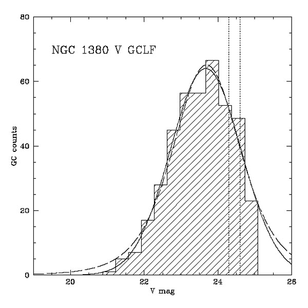 |
Figure 8. Typical GCLF, observed in the V band in the galaxy NGC 1380 (Della Valle et al. 1998). Over-plotted are two fits (a Gaussian and a student t5 function). The dotted lines show the 50% completeness limit in the V filter and in the filter combination (B, V, R) that was used to select the globular clusters. The apparent peak magnitude can be derived and the distance computed using the absolute magnitude obtained from local or secondary calibrators. |
The justification of the method is mainly empirical. Apparent turn-overs for galaxies at the same distance (e.g. in the same galaxy cluster) can be compared and a scatter around 0.15 mag is then obtained, without correcting for any external error. Similarly, a number of well observed apparent turn-over magnitudes can be transformed into absolute ones using distances from other distance indicators (Cepheids where possible, or a mean of Cepheids, surface brightness fluctuations, planetary luminosity function, ...) and a similar small scatter is found (see Harris 2000 for a recent compilation). Taking into account the errors in the photometry, the fitting of the GCLF, the assumed distances, etc... this hintsat an internal dispersion of the turn-over magnitude of < 0.1, making it a good standard candle. From a theoretical point of view, this constancy of the turn-over magnitude translates into a "universal" characteristic mass in the globular cluster mass distributions in all galaxies. Whether this is a relict of a characteristic mass in the mass function of the molecular clouds at the origin of the globular clusters, or whether it was implemented during the formation process of the globular clusters is still unclear.
The absolute turn-over magnitude lies around VTO ~ -7.5, and the determination of the visual turn-over is only accurate if the peak of the GCLF is reached by the observations. From an observational point of view, this means that the data must reach e.g. V ~ 25 to determine distances in the Fornax or Virgo galaxy clusters (D ~ 20 Mpc), and that with HST or 10m-class telescopes reaching typically V ~ 28, the method could be applied as far out as 120 Mpc (including the Coma galaxy cluster).
The observational advantages of this method over others are that globular clusters are brighter than other standard candles (except for supernovae), and do not vary, i.e. no repeated observations are necessary. Further, they are usually measured at large radii or in the halo of (mostly elliptical) galaxies where reddening is not a concern.
A large number of distance determinations from the GCLF were only by-products of globular cluster system studies, and often suffered from purely practical problems of data taken for different purposes.
First, a good estimation of the background contamination is necessary to clean the globular cluster luminosity function from the luminosity function of background galaxies which tends to mimic a fainter turn-over magnitude. Next, the finding incompleteness for the globular clusters needs to be determined, in particular as a function of radius since the photon noise is changing dramatically with galactocentric radius. Proper reddening corrections need to be applied and might differ whether one uses the "classical" reddening maps of Burstein & Heiles (1984) or the newer maps from Schlegel et al. (1998). When necessary, proper aperture correction for slightly extended clusters on WFPC2/HST images has to be made (e.g. Puzia et al. 1999). Finally, several different ways of fitting the GCLF are used: from fitting a histogram, over more sophisticated maximum-likelihood fits taking into account background contamination and incompleteness. The functions fitted vary from Gaussians to Student (t5) functions, with or without their dispersion as a free parameter in addition to the peak value.
In addition to these, errors in the absolute calibration will be added (see below). Furthermore, dependences on galaxy type and environment were claimed, although the former is probably due to the mean metallicity of globular clusters differing in early- and late-type galaxies, while the latter was never demonstrated with a reliable set of data.
All the above details can introduce errors in the analysis that might sum up to several tenths of a magnitude. The fact that distance determinations using the GCLF are often a by-product of studies aiming at understanding globular cluster or galaxy formation and evolution, did not help in constructing a very homogeneous sample in the past. The result is a very inhomogeneous database (e.g. Ferrarese et al. 1999) dominated by large random scatter introduced in the analysis, as well as systematic errors introduced by the choice of calibration and the complex nature of globular cluster systems (see below). Nevertheless, most of these problems were recognized and are overcome by better methods and data in the recent GCLF distance determinations.
7.3. The classical way: using all globular clusters of a system
Harris (2000, see also Kavelaars et al. 2000) outline what we will call the classical way of measuring distances with the GCLF. This method implies that the GCLF is measured from all globular clusters in a system. In addition, it uses the GCLF as a "secondary" distance indicator, basing its calibration on distances derived by Cepheids an other distance indicators. The method compares the peak of the observed GCLF with the peak of a compilation of GCLFs from mostly Virgo and Fornax ellipticals, adopting from the literature a distance to these calibrators. This allowed, among others, Harris' group to determine a distance to Coma ellipticals and to construct the first Hubble diagram from GCLFs in order to derive a value for H0 (Harris 2000, Kavelaars et al. 2000).
In practice, an accurate GCLF turn-over is determined (see above) and calibrated without any further corrections using MV(TO) = -7.33 ± 0.04 (Harris 2000) or MV(TO) = -7.26 ± 0.06 using Virgo alone (Kavelaars et al. 2000).
The advantages of this approach are the following. Using all globular clusters (instead of a limited sub-population) often avoids problems with small number statistics. This is also the idea behind using Virgo GCLFs instead of the spars Milky Way GCLF as calibrators. The Virgo GCLFs, derived from giant elliptical galaxies rich in globular clusters, are well sampled and do not suffer from small number statistics. Further, since most newly derived GCLFs come from cluster ellipticals, one might be more confident to calibrate these using Virgo (i.e. cluster) ellipticals, in order to avoid any potential dependence on galaxy type and/or environment.
However, the method has a number of caveats. The main one is that giant ellipticals are known to have globular cluster sub-populations with different ages and metallicities. This automatically implies that the different sub-populations around a given galaxy will have different turn-over magnitudes. By using the whole globular cluster systems, one is using a mix of turn-over magnitudes. One could in principal try to correct e.g. for a mean metallicity (as proposed by Ashman, Conti & Zepf 1995), but this correction depends on the population synthesis model adopted (see Puzia et al. 1999) and implies that the mix of metal-poor to metal-rich globular clusters is known. This mix does not only vary from galaxy to galaxy (e.g. Gebhardt & Kissler-Patig 1999), but also varies with galactocentric radius (e.g. Geisler et al. 1996, Kissler-Patig et al. 1997). It results in a displacement of the turn-over peak and the broadening of the observed GCLF of the whole system. The Virgo ellipticals are therefore only valid calibrators for other giant ellipticals with a similar ratio of metal-poor to metal-rich globular clusters and for which the observations cover similar radii. This is potentially a problem when comparing ground-based (wide-field) studies with HST studies focusing on the inner regions of a galaxy. Or when comparing nearby galaxies where the center is well sampled to very distant galaxies for which mostly halo globulars are observed. In the worse case, ignoring the presence of different sub-populations and comparing very different galaxies in this respect, can introduce errors a several tenths of magnitudes.
Another caveat of the classical way, is that relative distances to Virgo can be derived, but absolute magnitudes (and e.g. values of H0) will still dependent on other methods such as Cepheids, surface brightness fluctuations (SBF), Planetary Nebulae luminosity functions (PNLF), and tip of red-giant branches (TRGB), i.e. the method will never overcome these other methods in accuracy and carry along any of their potential systematic errors.
7.4. The alternative way: using metal-poor globular clusters only
As an alternative to the classical way, one can focus on the metal-poor clusters only. The idea is to isolate the metal-poor globular clusters of a system and to determine their GCLF. As a calibrator, one can use the GCLF of the metal-poor globular clusters in the Milky Way, which avoids any assumption on the distance of the LMC and will be independent of any other extragalactic distance indicator. For the Milky Way GCLF, the idea is to re-derive an absolute distance to each individual cluster, resulting in individual absolute magnitudes and allowing to derive an absolute luminosity function. Individual distances to the clusters are derived using the known apparent magnitudes of their horizontal branches and a relation between the absolute magnitude of the horizontal branch and the metallicity (e.g. Gratton et al. 1997). The latter is based on HIPPARCOS distances to sub-dwarfs fitted to the lower main sequence of chosen clusters. This methods follows a completely different path than methods based at some stage on Cepheids. In particular, the method is completely independently from the distance to the LMC.
In practice, an accurate GCLF turn-over (see above) for the metal-poor clusters in the target galaxy is derived and calibrated, without any further corrections, using MV(TO) = -7.62 ± 0.06 derived from the metal-poor clusters of the Milky Way (see Della Valle et al. 1998, Drenkhahn & Richtler 1999; note that the error is statistical only and does not include any potential systematic error associated with the distance to Galatic globular clusters, currently under debate).
The advantages of this method are the following. This method takes into account the known sub-structures of globular cluster systems. Using the metal-poor globular clusters is motivated by several facts. First, they appear to have a true universal origin (see Burgarella et al. 2000), and their properties seem to be relatively independent of galaxy type, environment, size and metallicity. Thus, to first order they can be used in all galaxies without applying any corrections. In addition, the Milky Way is justified as calibrator even for GCLFs derived from elliptical galaxies. Further, they appear to be "halo" objects, i.e. little affected by destruction processes that might have shaped the GCLF in the inner few kpc of large galaxies, or that affect objects on radial orbits. They will certainly form a much more homogeneous populations than the total globular cluster system (see previous sections). Using the Milky Way as calibrator allows this method to be completely independent on other distance indicators and to check independently derived distances and value of H0.
The method is not free from disadvantages. First, selecting metal-poor globular clusters requires better data than are currently used in most GCLF studies, implying more complicated and time-consuming observations. Second, even with excellent data a perfect separation of metal-poor and metal-rich clusters will not be possible and the sample will be somewhat contaminated by metal-rich clusters. Worse, the sample size will be roughly halved (for a typical ratio of blue to red clusters around one). This might mean that in some galaxies less than hundred clusters will be available to construct the luminosity function, inducing error > 0.1 on the peak determination due to sample size alone. Finally, the same concerns applies as for the whole sample: how universal is the GCLF peak of metal-poor globular clusters? This remains to be checked, but since variations of the order of < 0.1 seem to be the rule for whole samples, there is no reason to expect a much larger scatter for metal-poor clusters alone.
7.5. A few examples, comparisons, and the value of H0 from the GCLF method
Two examples of distance determinations from metal-poor clusters were given in Della Valle et al. (1998), and Puzia et al. (1999).
The first study derived a distance modulus for NGC 1380 in the Fornax cluster of (m - M) = 31.35 ± 0.09 (not including a potential systematic error of up to 0.2). In this case, the GCLF of the metal-poor and the metal-rich clusters peaked at the same value, i.e. the higher metallicity was compensated by a younger age (few Gyr) of the red globular cluster population, so that it would not make a difference whether one uses the metal-poor clusters alone or the whole system. As a comparison, values derived from Cepheids and a mean of Cepheids/SBF/PNLF to Fornax are (m - M) = 31.54 ± 0.14 (Ferrarese et al. 1999) and (m - M) = 31.30 ± 0.04 (from Kavelaars et al. 2000).
In the case of NGC 4472 in the Virgo galaxy cluster, Puzia et al. (1999) derived turn-overs from the metal-poor and metal-rich clusters of 23.67 ± 0.09 and 24.13 ± 0.11 respectively. Using the metal-poor clusters alone, their derived distance is then (m - M) = 30.99 ± 0.11. This compares with the Cepheid distance to Virgo from 6 galaxies of (m - M) = 31.01 ± 0.07 and to the mean of Cepheids/SBF/TRGB/PNLF of (m - M) = 30.99 ± 0.04 (from Kavelaars et al. 2000). Both cases show clearly the excellent agreement of the GCLF method with other popular methods, despite the completely different and independent calibrators used. The accuracy of the GCLF method will always be limited by the sample size and lies around ~ 0.1.
A nice example of the "classical way" is the recent determination of the distance to Coma. At the distance of ~ 100 Mpc the separation of metal-poor and metal-rich globular clusters is barely feasible anymore, and using the full globular cluster systems is necessary. Kavelaars et al. (2000) derived turn-over values of MV(TO) = 27.82 ± 0.13 and MV(TO) = 27.72 ± 0.20 for the two galaxies NGC 4874 and IC 4051 in Coma, respectively. Using Virgo ellipticals as calibrators and assuming a distance to Virgo of (m - M) = 30.99 ± 0.04, they derive a distance to Coma of 102 ± 6 Mpc. Adding several turn-over values for distant galaxies (taken from Lauer et al. 1998), they construct a Hubble diagram for the GCLF technique and derive a Hubble constant of H0 = 69 ± 9 km s-1 Mpc-1. This example demonstrates the reach in distance of the method.
In summary, we think that the method is mature now and that most errors in the analysis can be avoided, as well as good choices for the calibration made. In the future, with HST and 10m-class telescope data, a number of determinations in the 100 Mpc range will emerge, and eventually, using metal-poor globular clusters only, this will give us a grasp on the distance scale completely independent from distances based at some stage on the LMC distance or Cepheids.