


3.1. The general problem and its solution
The general problem of Bayesian parameter inference can be
specified as follows. We first choose a model containing a set of
hypotheses in the form of a vector of parameters,
 . The
parameters might describe any aspect of the model, but usually
they will represent some physically meaningful quantity, such as
for example the mass of an extra-solar planet or the abundance of
dark matter in the Universe. Together with the model we must
specify the priors for the parameters. Priors should summarize our
state of knowledge about the parameters before we consider the new
data, and for the parameter inference step the prior for a new
observation might be taken to be the posterior from a previous
measurement (for model comparison issues the prior is better
understood in a different way, see section 4).
The caveats about priors and prior specifications presented in
the previous section will apply at this stage.
. The
parameters might describe any aspect of the model, but usually
they will represent some physically meaningful quantity, such as
for example the mass of an extra-solar planet or the abundance of
dark matter in the Universe. Together with the model we must
specify the priors for the parameters. Priors should summarize our
state of knowledge about the parameters before we consider the new
data, and for the parameter inference step the prior for a new
observation might be taken to be the posterior from a previous
measurement (for model comparison issues the prior is better
understood in a different way, see section 4).
The caveats about priors and prior specifications presented in
the previous section will apply at this stage.
The central step is to construct the likelihood function for the
measurement, which usually reflects the way the data are obtained.
For example, a measurement with Gaussian noise will be represented
by a Normal distribution, while
 -ray
counts on a detector
will have a Poisson distribution for a likelihood. Nuisance
parameters related to the measurement process might be present in
the likelihood, e.g. the variance of the Gaussian might be unknown
or the background rate in the absence of the source might be
subject to uncertainty. This is no matter of concern for a
Bayesian, as the general strategy is always to work out the joint
posterior for all of the parameters in the problem and then
marginalize over the ones we are not interested in. Assuming that
we have a set of physically interesting parameters ϕ and a
set of nuisance parameters
-ray
counts on a detector
will have a Poisson distribution for a likelihood. Nuisance
parameters related to the measurement process might be present in
the likelihood, e.g. the variance of the Gaussian might be unknown
or the background rate in the absence of the source might be
subject to uncertainty. This is no matter of concern for a
Bayesian, as the general strategy is always to work out the joint
posterior for all of the parameters in the problem and then
marginalize over the ones we are not interested in. Assuming that
we have a set of physically interesting parameters ϕ and a
set of nuisance parameters
 , the joint posterior for
= (ϕ,
) is obtained through Bayes'
Theorem:
, the joint posterior for
= (ϕ,
) is obtained through Bayes'
Theorem:
 |
(12) |
where we have made explicit the choice of a model
 by
writing it on the righ-hand-side of the conditioning symbol.
Recall that
by
writing it on the righ-hand-side of the conditioning symbol.
Recall that  ( )
( )
 p(d |
,
)
denotes the likelihood and
p(|
) the prior. The
normalizing constant p(d |
) ("the Bayesian evidence")
is irrelevant for parameter inference (but central to model
comparison, see section 4), so we can write the
marginal posterior on the parameter of interest as (marginalizing
over the nuisance parameters)
p(d |
,
)
denotes the likelihood and
p(|
) the prior. The
normalizing constant p(d |
) ("the Bayesian evidence")
is irrelevant for parameter inference (but central to model
comparison, see section 4), so we can write the
marginal posterior on the parameter of interest as (marginalizing
over the nuisance parameters)
 |
(13) |
The final inference on ϕ from the posterior can then be communicated either by some summary statistics (such as the mean, the median or the mode of the distribution, its standard deviation and the correlation matrix among the components) or more usefully (especially for cases where the posterior presents multiple peaks or heavy tails) by plotting one or two dimensional subsets of ϕ, with the other components marginalized over.
In real life there are only a few cases of interest for which the above procedure can be carried out analytically. Quite often, however, the simple case of a Gaussian prior and a Gaussian likelihood can offer useful guidance regarding the behaviour of more complex problems. An analytical model of a Poisson-distributed likelihood for estimating source counts in the presence of a background signal is worked out in [14]. In general, however, actual problems in cosmology and astrophysics are not analytically tractable and one must resort to numerical techniques to evaluate the likelihood and to draw samples from the posterior. Fortunately this is not a major hurdle thanks to the recent increase of cheap computational power. In particular, numerical inference often employs a technique called Markov Chain Monte Carlo, which allows to map out numerically the posterior distribution of Eq. (12) even in the most complicated situations, where the likelihood can only be obtained by numerical simulation, the parameter space can have hundreds of dimensions and the posterior has multiple peaks and a complicated structure.
For further reading about Bayesian parameter inference, see [29, 10, 30, 11]. For more advanced applications to problems in astrophysics and cosmology, see [31, 16].
3.2. Markov Chain Monte Carlo techniques for parameter inference
The general solution to any inference problem has been outlined in the section above: it remains to find a way to evaluate the posterior of Eq. (12) for the usual case where analytical solutions do not exist or are insufficiently accurate. Nowadays, Bayesian inference heavily relies on numerical simulation, in particular in the form of Markov Chain Monte Carlo (MCMC) techniques, which are discussed in this section.
The purpose of the Markov chain Monte Carlo algorithm is to
construct a sequence of points in parameter space (called "a
chain"), whose density is proportional to the posterior pdf of
Eq. (12). Developing a full theory of Markov
chains is beyond the scope of the present article (see e.g.
[32,
33]
instead). For our purposes
it suffices to say that a Markov chain is defined as a sequence of
random variables {X(0), X(1), ...,
X(M-1)} such
that the probability of the (t + 1)-th element in the chain only
depends on the value of the t-th element. The crucial property
of Markov chains is that they can be shown to converge to a
stationary state (i.e., which does not change with t) where
successive elements of the chain are samples from the target
distribution, in our case the posterior
p(|d). The
generation of the elements of the chain is probabilistic in
nature, and several algorithms are available to construct Markov
chains. The choice of algorithm is highly dependent on the
characteristics of the problem at hand, and "tayloring" the MCMC
to the posterior one wants to explore often takes a lot of effort.
Popular and effective algorithms include the Metropolis-Hastings algorithm
[34,
35],
Gibbs sampling (see e.g.
[36]),
Hamiltonian Monte Carlo (see e.g.
[37]
and importance sampling.
Once a Markov chain has been constructed, obtaining Monte Carlo estimates of expectations for any function of the parameters becomes a trivial task. For example, the posterior mean is given by (where < ⋅ > denotes the expectation value with respect to the posterior)
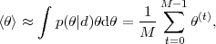 |
(14) |
where the equality with the mean of the samples from the MCMC
follows because the samples
(t)
are generated from the
posterior by construction. In general, one can easily obtain the
expectation value of any function of the parameters
f()
as
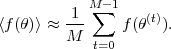 |
(15) |
It is usually interesting to summarize the results of the
inference by giving the 1-dimensional marginal probability
for the j-th element of , j.
Taking without
loss of generality j = 1 and a parameter space of dimensionality
n, the equivalent expression to
Eq. (3) for the case of continuous variables is
 |
(16) |
where
p(1
| d) is the marginal posterior for the
parameter 1.
From the Markov chain it is trivial to obtain and plot the marginal
posterior on the left-hand-side of Eq. (16): since the elements of
the Markov chains are samples from the full posterior,
p(|d),
their density reflects the value of the full
posterior pdf. It is then sufficient to divide the range of
1 in a series
of bins and count the number of
samples falling within each bin, simply ignoring the coordinates
values 2,
..., n. A
2-dimensional posterior is defined in an analogous fashion.
There are several important practical issues in working with MCMC methods (for details see e.g. [32]). Especially for high-dimensional parameter spaces with multi-modal posteriors it is important not to use MCMC techniques as a black box, since poor exploration of the posterior can lead to serious mistakes in the final inference if it remains undetected. Considerable care is required to ensure as much as possible that the MCMC exploration has covered the relevant parameter space.