6. COSMOLOGICAL BAYESIAN MODEL BUILDING

The Bayesian model comparison approach based on the evaluation of the evidence is being increasingly applied to model building questions such as: are isocurvature contributions to the initial conditions required by the data [46, 58, 60, 182]? Is the Universe flat [183, 58, 70]? What is the best description of the primordial power spectrum for density perturbations [51, 184, 58, 185, 165, 47, 70]? Is dark energy best described as a cosmological constant [186, 50, 51, 187, 188, 189, 190, 191]? In this section we review the status of the field.

6.1. Evidence for the cosmological concordance model

Table 4 is a fairly extensive compilation of recent results regarding possible extensions to (or reduction of) the vanilla CDM concordance cosmological model introduced in section 5.1. We have chosen to compile only results obtained using the full Bayesian evidence, rather than approximate model comparisons obtained via the information criteria because the latter are often not adequate approximations, for the reasons explained in section 4.7. Of course, the outcome depends on the Occam's razor effect brought about by the prior volume (and sometimes, by the choice of parameterization). Where applicable, we have show the sensitivity of the result on the prior assumptions by giving a ballpark range of values for the Bayes factor, as presented in the original studies. The reader ought to refer to the original works for the precise prior and parameter choices and for the justification of the assumed prior ranges.

Table 4. Summary of model comparison results against the CDM concordance model (see Table 3) using Bayesian model comparison for nested models. A negative (positive) value for ln B indicates that the competing model is disfavoured (supported) with respect to the CDM model. The column N_par gives the difference in the number of free parameters with respect to the CDM concordance model. A negative value means that one of the parameters has been fixed. See references for full details and in particular for the choice of priors on the model parameters, which control the strengths of the Occam's razor effect.

Competing model	Npar	ln B	Ref	Data	Outcome
Initial conditions
Isocurvature modes
CDM isocurvature	+1	-7.6	[58]	WMAP3+, LSS	Strong evidence for adiabaticity
+ arbitrary correlations	+4	-1.0	[46]	WMAP1+, LSS, SN Ia	Undecided
Neutrino entropy	+1	[-2.5, -6.5]p	[60]	WMAP3+, LSS	Moderate to strong evidence for adiabaticity
+ arbitrary correlations	+4	-1.0	[46]	WMAP1+, LSS, SN Ia	Undecided
Neutrino velocity	+1	[-2.5, -6.5]p	[60]	WMAP3+, LSS	Moderate to strong evidence for adiabaticity
+ arbitrary correlations	+4	-1.0	[46]	WMAP1+, LSS, SN Ia	Undecided
Primordial power spectrum
No tilt (ns = 1)	-1	+0.4	[47]	WMAP1+, LSS	Undecided
		[-1.1, -0.6]p	[51]	WMAP1+, LSS	Undecided
		-0.7	[58]	WMAP1+, LSS	Undecided
		-0.9	[70]	WMAP1+	Undecided
		[-0.7, -1.7]p,d	[185]	WMAP3+	ns = 1 weakly disfavoured
		-2.0	[184]	WMAP3+, LSS	ns = 1 weakly disfavoured
		-2.6	[70]	WMAP3+	ns = 1 moderately disfavoured
		-2.9	[58]	WMAP3+, LSS	ns = 1 moderately disfavoured
		<-3.9c	[65]	WMAP3+, LSS	Moderate evidence at best against ns ≠ 1
Running	+1	[-0.6, 1.0]p,d	[185]	WMAP3+, LSS	No evidence for running
		< 0.2c	[165]	WMAP3+, LSS	Running not required
Running of running	+2	<0.4c	[165]	WMAP3+, LSS	Not required
Large scales cut-off	+2	[1.3, 2.2]p,d	[185]	WMAP3+, LSS	Weak support for a cut-off
Matter-energy content
Non-flat Universe	+1	-3.8	[70]	WMAP3+, HST	Flat Universe moderately favoured
		-3.4	[58]	WMAP3+, LSS, HST	Flat Universe moderately favoured
Coupled neutrinos	+1	-0.7	[192]	WMAP3+, LSS	No evidence for non-SM neutrinos
Dark energy sector
w(z)= weff ≠ -1	+1	[-1.3, -2.7]p	[186]	SN Ia	Weak to moderate support for
		-3.0	[50]	SN Ia	Moderate support for
		-1.1	[51]	WMAP1+, LSS, SN Ia	Weak support for
		[-0.2, -1]p	[187]	SN Ia, BAO, WMAP3	Undecided
		[-1.6, -2.3]d	[188]	SN Ia, GRB	Weak support for
w(z) = w0 + w1 z	+2	[-1.5, -3.4]p	[186]	SN Ia	Weak to moderate support for
		-6.0	[50]	SN Ia	Strong support for
		-1.8	[187]	SN Ia, BAO, WMAP3	Weak support for
w(z) = w0 + wa(1 - a)	+2	-1.1	[187]	SN Ia, BAO, WMAP3	Weak support for
		[-1.2, -2.6]d	[188]	SN Ia, GRB	Weak to moderate support for
Reionization history
No reionization ( = 0)	-1	-2.6	[70]	WMAP3+, HST	≠ 0 moderately favoured
No reionization and no tilt	-2	-10.3	[70]	WMAP3+, HST	Strongly disfavoured
d Depending on the choice of datasets.
p Depending on the choice of priors.
c Upper bound using Bayesian calibrated p-values, see section 4.5. Data sets: WMAP1+ (WMAP3+): WMAP 1st year (3-yr) data and other CMB measurements. LSS: Large scale structures data. SN Ia: supernovae type Ia. BAO: baryonic acoustic oscillations. GRB: gamma ray bursts.

As anticipated, the 6 parameters CDM concordance model is currently well supported by the data, as the inclusion of extra parameters is not required by the Bayesian evidence. This is shown by the fact that most model comparisons return either an undecided result or they support the CDM model (negative values for ln B in Table 4). The only exception is the support for a cut-off on large scales in the power spectrum reported by [185]. This is clearly driven by the anomalies in the large scale CMB power spectrum, which in this case are interpreted as being a reflection of a lack of power in the primordial power spectrum. Whether such anomalies are of cosmological origin remains however an open question [193, 194]. If extensions of the model are not supported, reduction of CDM to simpler models is not viable, either: recent studies employing WMAP 3-yr data find that a scale invariant spectrum with no spectral tilt is now weakly to moderately disfavoured [184, 70, 58, 65]. Also, a Universe with no reionization is no longer a good description of CMB data, and a non-zero optical depth is indeed required [70].

A few further comments about the results reported in Table 4 are in place:

1. Regarding the type of initial conditions for cosmological perturbations, all parameter extraction studies to date (with the exception of [195]) find that a purely adiabatic mode is in agreement with observations, and constrain the isocurvature fraction to be below about 10% for one single isocurvature mode at the time [60] and below about 50% for a general mixture of modes [196, 197]. From a model selection perspective, this means that we expect the purely adiabatic model to be preferred over a more complex model with a mixture of isocurvature modes. This is indeed the case, but the result is strongly dependent on the parameterization adopted for the isocurvature sector, which determines the strength of the Occam's razor effect. This is a consequence of the difficulty of coming up with a well motivated phenomenological parameterization of the isocurvature amplitudes, see the discussion in [58, 182].
2. The shape of the primordial power spectrum has attracted considerable attention from a model comparison perspective [47, 51, 58, 70, 185, 184, 65, 165]. With the exception of the large scale cut-off mentioned above, the current consensus appears to be that a power-law distribution of fluctuations, with power spectrum P(k) = P₀ (k / k₀)^n_s-1 with n_s < 1 is currently the best description. This is usually interpreted as evidence for inflation. However, a proper model comparison of inflationary predictions involves including the presence of tensor modes generated by gravitational waves, parameterized in terms of their amplitude parameter r. Including this extra parameter runs into the difficulty of specifying its prior volume, as the two obvious choices of priors flat in r or logr lead to very different model comparison results [184]. Another problem is that the comparison might be ill-defined, as the simpler model with n_s = 1 and r = 0 is presumably some sort of alternative, unspecified model without inflation that would not solve the horizon problem. On this ground alone, unless an alternative solution to the horizon problem is put on the table, such an alternative model would be immediately thrown out (see the discussion in [165]). Finally, higher-order terms in the Taylor expansion of the power spectrum, such as a running of the spectral index or a running of the running, are currently not required. This appears a robust result with respect to a wide choice of priors and data sets.
3. Present-day constraints on the curvature of spatial sections are of order || 0.01 (with = 0 corresponding to a flat, Euclidean geometry), stemming from a combination of CMB, large scale structures and supernovae data. Choosing a phenomenological prior of width = 1 around 0 delivers a moderate support for a flat Universe versus curved models [70, 58]. However, adopting an inflation-motivated prior instead, ~ 10^-5, would lead to an undecided result (ln B = 0) for the model comparison, as the data are not strong enough to discriminate between the two models in this case. This can be formalized by considering the Bayesian model complexity for the two choices of priors, Eq. (35). Noticing that / is the ratio between the likelihood and prior widths, for a prior on the curvature parameter of width 1, / ~ 10^-2 and _b ≈ 1, hence the parameter has been measured. But if we take a prior width ~ 10^-5, / ~ 10³ hence _b → 0. In the latter case, we can see from Eq. (21) that the Bayes factor between the two models B₀₁ → 1 and the evidence is inconclusive, awaiting better data.
4. Model comparisons regarding the dark energy sector suffer from considerably uncertainty. Clearly, the model to beat is the cosmological constant (with equation of state parameter w =-1 at all redshifts), but alternative dark energy scenarios suffer from the fundamental difficulty of motivating physically both the parameterization of the dark energy time dependence and the prior volume for the extra parameters [198] (see [199] for a review of models and [200] for on overview of recent constraints). However, the semi-phenomenological studies shown in Table 4 do agree in deeming a cosmological constant a sufficient description of the data. This is again a consequence of the fact that no time evolution of the equation of state is detected in the data, hence the strength of the support in favour of the cosmological constant becomes a function of the available parameter space under the more complex, alternative models. Given this result, it is interesting to ask what level of accuracy is required before our degree of belief in the cosmological constant is overwhelmingly larger than for an evolving dark energy, assuming of course that future data will not detect any significant departure from w = -1. To this end, a simple classification of models has been given in [201] in terms of their effective equation of space parameter, w_eff, representing the time-varying equation of state averaged over redshift with the appropriate weighting factor for the observable [202]. The three categories considered are "phantom models" (exhibiting large, negative values for the equation of state, -11 w_eff -1), "fluid-like dark energy" (-1 w_eff -1/3) and "small-departures from " models (-1.01 w_eff 0.99). Assuming a flat prior on these ranges of values for w_eff, consideration of the Bayes factor between each of those models and the cosmological constant shows that gathering strong evidence against each of the models requires an accuracy on w_eff of order _eff = 0.05 for phantom models (which are therefore already under pressure from current data, which have an accuracy of order ~ 0.1), _eff = 3 × 10^-3 for fluid-like models (about a factor of 5 better than optimistic constraints from future observations) and _eff = 5 × 10^-5 for small-departure models. Refinements of this approach that employ more fundamentally-motivated priors could lead to an analysis of the expected costs/benefits from future dark energy observations in terms of their likely model selection outcome (we return on this issue in section 6.2).

Let us now turn to models that are not nested within CDM— i.e., alternative theoretical scenarios. Table 5 gives some examples of the outcome of the Bayesian model comparison with the concordance model. As above, we restrict our considerations to studies employing the full Bayesian evidence (there are many other examples in the literature carrying out approximate model comparison using information criteria instead). The model comparison is often more difficult for non-nested models, as priors must be specified for all of the parameters in the alternative model (and in the CDM model, as well), in order to compute the evidence ratio. The usual caveats on prior choice apply in this case. From Table 5 it appears that the data do not seem to require fundamental changes in our underlying theoretical model, either in the form of Bianchi templates representing a violation of cosmic isotropy (see also [206]), or as Lemaitre-Tolman-Bondi models or fractal bubble scenarios with dressed cosmological parameters. The anomalous dipole in the CMB temperature maps is a fine example of Lindley's paradox. When fitting a dipolar template to the CMB maps, the effective chi-square improves by 9 to 11 units (depending on the details of the analysis) for 3 extra parameters [205, 207], which would be deemed a "significant" effect using a standard goodness-of-fit test. However, the Bayesian evidence analysis shows that the odds in favour of an anomalous dipole are 9 to 1 at best (corresponding to ln B < 2.2), which does not reach the "moderate evidence at best" threshold. Hence Bayesian model comparison is conservative, requiring a stronger evidence before deeming an effect to be favoured.

Table 5. Summary of model comparison results against the CDM concordance model for some alternative (i.e., non-nested) cosmological models. A negative (positive) value for ln B indicates that the competing model is disfavoured (supported) with respect to CDM. The column N_par gives the number of free parameters in the alternative model. See references for full details about the models, priors and data used.

Competing model	Npar	ln B	Ref	Data	Outcome
Alternatives to FRW
Bianchi VIIh	5 to 8	[-0.9, 1.2]d,p	[54]	WMAP1, WMAP3	Weak support (at best) for Bianchi template
	5 to 6	[-0.1, -1.2]p	[203]	WMAP3	No evidence after texture correction
LTB models	4	-3.6	[204]	WMAP3, BAO, SN Ia	Moderate evidence against LTB
Fractal bubble model	2	0.3	[89]	SN Ia	Undecided
Asymmetry in the CMB
Anomalous dipole	3	1.8	[205]	WMAP3	Weak evidence for anomalous dipole
		< 2.2c	[65]	WMAP3	Weak evidence at best
d Depending on the choice of datasets.
p Depending on the choice of priors.
c Upper bound using Bayesian calibrated p-values, see section 4.5.

6.2. Other uses of the Bayesian evidence

Beside cosmological model building, the Bayesian evidence can be employed in many other different ways. Here we presents two aspects that are relevant to our topic, namely the applications to the field of multi-model inference and model selection forecasting.

1. Multi-model inference. Once we realize that there are several possible models for our data, it becomes interesting to present parameter inferences that take into account the model uncertainty associated with this plurality of possibilities. In other words, instead of just constraining parameters within each model, we can take a step further and produce parameter inferences that are averaged over the models being considered. Let us suppose that we have a minimal model (in our case, CDM) and a series of augmented models with extra parameters. A typical example from cosmology is dark energy (first discussed in the context of multi-model averaging in [208]), where the minimal model has w = -1 fixed and there are several other candidate models with a time-varying equation of state, parameterized in terms of a number of free parameters and their priors. Let us denote by the cosmological parameters common to all models. For the extended models, the redshift-dependence of the dark energy equation of state is described by a vector of parameters _i (under model _i). The CDM model has no free parameters for the equation of state, hence the prior on _CDM is a delta function centered on w(z) = w₀ = -1. Then a straightforward application of Bayes' theorem leads to the following posterior distribution for the parameters:

   (48)

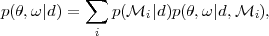
   where p(, | d, _i) is the posterior within each model _i, and it is understood that the posterior has non-zero support only along the parameter directions _i ⊂ that are relevant for the model, and delta-functions along all other directions. Each term is weighted by the corresponding posterior model probability,

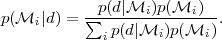   (49)

   The prior model probabilities p(_i) are usually set equal, but a model preference can be incorporated here if necessary. The model averaged posterior distribution of Eq. (48) then represents the parameter constraints obtained independently of the model choice, which has been marginalized over. Unless one of the models is overwhelmingly more probable than the others (in which case the model averaging essentially disappears, as all of the weights for the other models go to zero), the model-averaged posterior distribution can be significantly different from the model-specific distribution. A counter-intuitive consequence is that in the case of dark energy, the model-averaged posterior shows tighter constraints around w = -1 than any of the evolving dark energy models by itself. This comes about because CDM is the preferred model and hence much of the weight in the model-averaged posterior is shifted to the point w = -1 [208]. For further details on multi-model inference, see e.g. [209, 210].

2. Model selection forecasting. When considering the capabilities of future experiments, it is common stance to predict their performance in terms of constraints on relevant parameters, assuming a fiducial point in parameter space as the true model (often, the current best-fit model). While this is a useful indicator for parameter inference tasks, many questions in cosmology fall rather in the model comparison category. A notable example is again dark energy, where the science driver for many future multi-million-dollar probes is to detect possible departures from a cosmological constant, hence to gather evidence in favour of an evolving dark energy model. It is therefore preferable to assess the capabilities of future experiments by their ability to answer model selection questions.

   The procedure is as follows (see [211] for details and the application to dark energy scenarios). At every point in parameter space, mock data from the future observation are generated and the Bayes factor between the competing models is computed, for example between an evolving dark energy and a cosmological constant. Then one delimits in parameter space the region where the future data would not be able to deliver a clear model comparison verdict, for example | ln B | < 5 (evidence falling short of the "strong" threshold). The experiment with the smallest "model-confusion" volume in parameter space is to be preferred, since it achieves the highest discriminative power between models. An application of a related technique to the spectral index from the Planck satellite is presented in [212, 213].

   Alternatively, we can investigate the full probability distribution for the Bayes factor from a future observation. This allows to make probabilistic statements regarding the outcome of a future model comparison, and in particular to quantify the probability that a new observation will be able to achieve a certain level of evidence for one of the models, given current knowledge. This technique is based on the predictive distribution for a future observation, which gives the expected posterior on for an observation with experimental capabilities described by e (this might describe sky coverage, noise levels, target redshift, etc):

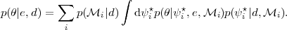   (50)

   Here, d are the currently available observations, p(_i | d) is the current model posterior, p( | _i^⋆, e, _i) is the posterior on from a future observation e computed assuming _i^⋆ are the correct model parameters, while each term is weighted by the present probability that _i^⋆ is the true value of the parameters, p(_i^⋆ | d, _i). The sum over i ensures that the prediction averages over models, as well. From Eq. (50) we can compute the corresponding probability distribution for ln B from experiment e, for example by employing MCMC techniques (further details are given in [59]). This method is called PPOD, for predictive posterior odds distribution and can be useful in the context of experiment design and optimization, when the aim is to determine which choice of e will lead to the best scientific return from the experiment, in this case in terms of model selection capabilities (see [214, 215, 216] for a discussion of performance optimization for parameter constraints). For further details on Bayes factor forecasts and experiment design, see [217].