


All calibrations and data reductions were performed using standard routines in the Common Astronomy Software Applications package, CASA 1, using versions 4.2 and earlier. Paper III describes in detail the process we have been following for calibrations and reductions. A summary follows here:
In order to reduce ringing across the band from strong RFI, it was necessary to Hanning smooth our data. Antenna-based delay calibrations have to be applied prior to this smoothing, which was done in an initial stage of the calibrations.
The absolute flux density scale of the data was determined by observing one of two standard primary calibrators; 3C286 or 33C48 (the latter for three of our early right ascension galaxies, NGC 891, NGC 660 and part of the NGC 2613 observations), and applying the Perley-Butler 2010 flux density scale. We used the primary calibrator to determine the bandpass corrections as well. See Table 1 for a list of the calibrators which were used for each galaxy in the sample.
3.1.1. Polarization calibration
For the polarization calibrations, the primary calibrator was used as a polarization angle calibrator. One of the NRAO standard zero polarization calibrators was used to calibrate instrumental polarization leakage. We corrected for cross-hand delays, leakage terms and polarization position angles. Where in some cases the polarization leakage calibrator could not be used (due to loss of scan during observation or being more heavily flagged than the other calibrators), we instead utilized the secondary calibrator where the range in parallactic angle was sufficient, i.e. more than 60 degrees. This was for example done for the galaxies in a C-band scheduling block (ID: 4809749), for which the polarization leakage calibrator scan was lost. Q and U fluxes were calculated in the standard way – see Paper II and references therein. Our tests have shown no difference in the result whether the secondary calibrator or polarization leakage calibrator was used.
For all scans, calibrators and galaxy scans alike, we inspected the uv-data by eye. All bad data, whether from RFI or instrumental effects, were manually flagged. A number of tests were carried out using automatic CASA flagging routines as well as the CASA pipeline; however, we found significantly improved results by continuing with manual flagging.
Generally, fewer antennas could be used for our L-band observations than for C-band, since not all VLA antennas had yet been equipped with L-band receivers at the time of observation. Additionally, there is typically more RFI at L-band.
Calibrations and flagging were carried out iteratively, until a well-calibrated data set could be obtained. The final calibrated galaxy scans were then separated from the calibrator scans, in order to be imaged in Stokes I, Q and U.
We have produced Stokes I, Q and U images, as well as spectral index maps (α, where Iν∝ να) and uncertainty maps, Δα (see Sect. 3.4) from the calibrated data.
The clean algorithm in CASA, which we use for our wide-field synthesis deconvolution, allows for multi-scale multi-frequency synthesis, ms-mfs (see Rau & Cornwell 2011, for a full description). We set the multi-scale feature to look for flux components at a variety of spatial scales, to account for the extended emission of our galaxies. Typically our scales ranged from zero (’classic clean’) up to approximately five times the synthesized beam, but sometimes required adjustments. In L-band, and for the uv-tapered weighting in particular, fewer scales were at times necessary in order to remove artifacts for point-like sources; for example a classic clean was set for NGC 2683, NGC 2992, NGC 4157 and NGC 4845.
Additionally, the clean algorithm enabled simultaneous fitting of a spectral index across the band width (’in-band spectral index’) via a simple power law. In order for this to take place, we set the number of Taylor coefficients used to model the sky frequency dependence,nterms, to 2 for all CHANG-ES galaxies. We defer the details of spectral information to Section 3.4, and will describe the spatial fitting, as implemented for the CHANG-ES project, in this section.
For each galaxy, the Briggs robust weighting (Briggs 1995) was used for both C and L band data. Additionally, we imaged a uv-tapered version of this weighting, which we introduced in order to emphasize the broadscale structures 2. We achieved an increase in beam size of approximately 80% in C-band and 40% in L-band, by typically applying a 6 kλ Gaussian taper in C-band and a 2.5 kλ Gaussian taper in L-band to the uv-distribution. Image products of both these weightings are included in Data Release 1 and are referred to as robust 0 and uv-tapered weightings, respectively.
In C-band, images sufficiently clear of artifacts with uv-tapered weighting could not be achieved for NGC 4438 and NGC 4845 due to particularly strong contaminating sources in the field. In L-band, the uv-tapered weighting was either challenging to achieve (for the same reason) or unnecessary (the sources were imaged as point sources already at robust 0) for six of our galaxies; NGC 3448, NGC 4192, NGC 4388, NGC 4438, NGC 4845 and UGC 10288, and the attempt was discarded for these. Hereafter any images shown will be of robust 0 weighting, unless otherwise specified.
Each imaging run was cleaned down to a flux density level of 2.5-3 σ. With few exceptions, we imaged the entire field (i.e. without specifying regions), since a lower rms could be obtained with this strategy. Additionally, the vast majority of our data do not suffer from significant artefact patterns with spurious sources outside the source region, which could jeopardize this strategy. When needed, one to two self calibrations were performed in order to deal with remaining artifacts.
Our self calibration strategy was based on iteratively refining the calibration table, by self calibrating at successively deeper thresholds and thus improving the input model, which in turn acts on the original visibilities. At each step, care was taken to a) check the model to be used for the self calibration that it did not include any artifacts and b) check that the peak intensity of the source would not decline (such a scenario was aided by opting for a phase-only self calibration at the first iteration, or by applying the self calibration at a shallower threshold).
In some cases, our cleaning strategy had to be adapted to the circumstances of the data (the quality of a dataset, strength of emission, contamination in the field, etc). This particularly applies to data with high dynamic ranges (HDR), due to galaxies with strong, often point-like centre sources or strong field sources (for example NGC 660, NGC 4594, Virgo galaxies). Our strategies to deal with these situations include one or more consecutive runs of self calibrations, specifying regions, attempts at peeling for strong field galaxies (see 3.3.6) and clean parameter adjustments (including multi-scale adjustments). Generally, the best one can achieve in terms of HDR, is a signal over noise of the order of 10000:1 (S. Bhatnagar, priv.comm.). Our dynamic ranges are listed in column 8 of Tables 4 and 5. Additionally, in cases of strong centre sources, choosing a smaller cell size will characterize the steep beam better and render a cleaner result (e.g. NGC 4594 and NGC 4845, both in C-band).
Stokes Q and U images were produced similarly to I. These maps were used to create polarization intensity and polarization angle maps. The polarization intensity maps were corrected for bias caused by the noise level 3 and the polarization angle maps are cut off at the 3σ level. We note that if the fraction of polarization intensity over Stokes I intensity is less than 0.5%, the polarization is not believable since the calibration cannot be guaranteed below that level (S. Myers, priv. comm.).
A uniform Faraday screen resulting from the ionosphere is corrected for in the standard polarization data reduction. However, if there is differential Faraday rotation, for example between the location of the primary calibrator and the source, then this is not corrected for 4. This effect is negligible at C-band. There could, however, be minor effects at L-band, which will be investigated in a subsequent polarization paper.
Our vector maps (panels (d), (e) and (f) of the figures in the appendix) are also ’apparent B-vectors’ which simply are E-vectors rotated by 90 degrees, because internal Faraday rotation in the galaxy has not been corrected for.
3.3.4. Primary beam corrections
Wideband primary beam corrections were carried out with the CASA task widebandpbcor after cleaning. This task accesses information about the beam from the visibility data, and calculates a known NRAO-supplied model of the primary beam (PB) at each frequency channel in each band. A PB cube is formed, and Taylor terms are found in the same way as was done for the data set when imaging. Each Taylor coefficient image (two in our case, see Sect. 3.3 and 3.4.1) is then corrected.
This task also corrects the spectral index image above a given threshold (we use 5σ), as well as corrects a map of the formal error of the spectral index (see Sec. 3.4.2). Subsequently, we also applied primary beam corrections to the polarization intensity maps, by dividing the image with the beam created in the widebandpbcor task.
Note that in this paper, any displayed images are not PB corrected, but any measurements are made from the PB-corrected versions of the maps, unless otherwise indicated. For total intensity images, use of a model for the PB rather than an observation-specific PB introduces negligible error over the scales of our galaxies. However, the effect on the spectral index maps must be investigated in more detail, which we do in Sec. 3.4.2.
3.3.5. Mosaicking two pointings
For the eight large galaxies which were observed in two pointings at C-band (see Table 2), each individual pointing was calibrated and imaged separately. Although it would be preferrable to mosaic the pointings onto the same grid while still in the uv-plane, this feature is not yet implemented in CASA at the time, for the clean settings that we required (i.e. nterms = 2). Instead, we combined the images from the two pointings, forming a weighted (by the primary beam) average in the overlapping region. The images were combined in the overlapping regions out to 10% of the primary beam. This rather inclusive choice of cut-off worked well for the D configuration data, but will likely be adjusted to 50% for the B and C configuration data in the future.
This strategy was applied to both the non-PB-corrected images, as well as the two primary beam pointings. The combined Stokes I image was divided by the combined primary beam in order to do the PB correction.
The two-pointing spectral index maps, which had already been individually PB-corrected, were similarly combined, as well as their accompanying error maps.
We assessed whether the two pointings had differences within the overlap regions, such as in noise levels. In such cases additional weightings, based on the noise level, would have to be considered. This was however not the case for any of the CHANG-ES galaxies, where separate pointings generally had been observed in turns in the same scheduling blocks, or in similar conditions.
3.3.6. Peeling of strong field sources
For a couple of cases, for example NGC 660 and NGC 4388, bright field sources interfere strongly in the cleaning process, causing a less than ideal imaging result fraught with severe artifacts (L-band only). An attempt was made at peeling these interfering sources in those examples, that is, to remove or decrease the intensity of the interfering source so that its impact is lessened in the final deconvolution. The process includes self calibrations with the interfering source centred, and subtracting the source from the uv-data using the CASA task uvsub, in several steps. For more information on peeling, see Pizzo & de Bruyn (2009), as well as the PhD thesis by Adebahr (2013). Table 3 lists the sources we peeled from NGC 660 and NGC 4438.
| Galaxy | Source name | Angular distance | Intensity before/after | RA | Dec |
| (') | (mJy/beam) | 1 | 2 | 3 | 4 | 5 | 6 |
| N660 | - | 15 | 95/26 | 01h 42m 18.8s | +13d 27m 48.6s |
| N4388 | M87 | 75 | 132/22 | 12h 30m 48s | +12d 23m 30.2s |
| NOTE. - Column 1: Galaxy name; Column 2: Name of interfering source 1; Column 3: distance in arcminutes between galaxy and interfering source; Column 4: Intensity of interfering source before/after peeling ; Column 5: Right Ascension; Column 6: Declination. | |||||
3.4.1. Formation of Spectral Index Maps
As indicated in Sect. 3.3, the ms-mfs algorithm allows for spectral fitting across the wide bands that have been used in the CHANG-ES survey. Thus, a single observation over a single wave-band permits the determination of spectral indices, α, as a function of position within the galaxy. As described in Rau & Cornwell (2011) (see also Paper II), a specific intensity, Iν, at some frequency, ν, within the band, can be fit with a function of the form Iν = Iν0 να +β log(ν/ν0), where β is a curvature term and ν0 is a reference frequency (our central frequency, ν0, given in Tables 4 and 5). As implemented, such a fitting function is expanded in a Taylor series about ν0, such that the first Taylor term (the map, TT0) corresponds to a map of specific intensities at ν0 and the second Taylor term (the map TT1) contains information on α such that α = TT1 / TT0. The third Taylor term (TT2) allows for the recovery of the spectral curvature, β, where β = TT2 / TT0 − α(α − 1)/2.
| Galaxy | weighting | Bmaj | Bmin | BPA | ν0 | rms I | Map peak | DR | rms QU | pol. peak |
| ["] | ["] | [degree] | [GHz] | [µJy/beam] | [mJy/beam] | [µJy/beam] | µJy/beam] | |||
| 1 | 2 | 3 | 4 | 5 | 6 | 7 | 8 | 9 | 10 | 11 |
| N660 | rob 0 | 9.55 | 9.14 | -18.72 | 5.99904 | 8.6 | 603 | 70116 | 6.0 | 369.1 |
| uvtap | 16.13 | 16 | -58.32 | 18 | 614 | 34111 | 7.0 | 554.6 | ||
| N891 | rob 0 | 9 | 8.81 | -79.46 | 5.99932 | 6.5 | 7.21 | 1109 | 6.6 | 115.0 |
| uvtap | 15.31 | 14.63 | 88.05 | 6.9 | 6.9 | 1000 | 7.2 | 225.0 | ||
| N2613 | rob 0 | 15.42 | 8.3 | -11.05 | 5.99900 | 10.1 | 0.643 | 64 | 10.4 | 57.1 |
| uvtap | 19.94 | 15.82 | -11.44 | 11.8 | 1.09 | 92 | 11.5 | 63.6 | ||
| N2683 | rob 0 | 9.36 | 8.76 | 11.71 | 5.99900 | 9.1 | 3.27 | 359 | 8.8 | 50.2 |
| uvtap | 15.88 | 14.81 | 46.67 | 9.4 | 3.31 | 352 | 8.9 | 64.6 | ||
| N2820 | rob 0 | 9.84 | 8.91 | -3.81 | 5.99900 | 5.3 | 1.699 | 321 | 5.3 | 48.7 |
| uvtap | 16.18 | 15.36 | -3.884 | 5.2 | 3.173 | 610 | 5.3 | 97.3 | ||
| N2992 | rob 0 | 14.33 | 8.84 | -13.3 | 5.99900 | 8.4 | 65.6 | 7810 | 8.0 | 151.7 |
| uvtap | 18.51 | 16.76 | -14.26 | 9.5 | 71.7 | 7547 | 8.2 | 202.8 | ||
| N3003 | rob 0 | 9.37 | 8.93 | -67.02 | 5.99900 | 9.4 | 1.35 | 144 | 8.6 | 41.1 |
| uvtap | 13.78 | 13.61 | 16.65 | 6.0 | 8.11 | 1352 | 9.2 | 40.0 | ||
| N3044 | rob 0 | 10.68 | 9.59 | -5.08 | 5.99900 | 5.1 | 5.92 | 1161 | 7.0 | 102.9 |
| uvtap | 13.78 | 13.61 | 16.65 | 6.0 | 8.11 | 1352 | 7.0 | 138.4 | ||
| N3079 | rob 0 | 9.32 | 8.72 | -13.89 | 5.99900 | 6.5 | 202.07 | 31088 | 5.9 | 1987.1 |
| uvtap | 16.16 | 15.44 | -9.5 | 8.0 | 221.93 | 27741 | 5.8 | 2759.5 | ||
| N3432 | rob 0 | 11.94 | 9.97 | 3.43 | 5.99900 | 7.2 | 2.33 | 324 | 7.1 | 39.2 |
| uvtap | 15 | 13.14 | -179.3 | 6.8 | 2.62 | 385 | 6.5 | 49.3 | ||
| N3448 | rob 0 | 9.1 | 8.6 | 3.4 | 5.99900 | 5.6 | 5.36 | 957 | 5.4 | 66.0 |
| uvtap | 16 | 15.7 | -167.6 | 6.6 | 8.46 | 1282 | 5.9 | 105.5 | ||
| N3556 | rob 0 | 9.2 | 8.7 | 7.6 | 5.99900 | 5.3 | 3.45 | 651 | 5.3 | 66.8 |
| uvtap | 16 | 15. | 14.1 | 6.0 | 6.9 | 1150 | 5.7 | 91.9 | ||
| N3628 | rob 0 | 9.62 | 9.47 | -31.09 | 5.99842 | 9.5 | 66.96 | 7048 | 10.2 | 174.2 |
| uvtap | 16.83 | 15.15 | 75.57 | 9.5 | 79.09 | 8325 | 9.6 | 128.4 | ||
| N3735 | rob 0 | 10.1 | 8.8 | -2.3 | 5.99900 | 5.8 | 2.9 | 500 | 5.6 | 109.5 |
| uvtap | 16.4 | 15.6 | -5 | 6.2 | 5.3 | 855 | 5.6 | 220.4 | ||
| N3877 | rob 0 | 8.85 | 8.66 | 39.45 | 5.99900 | 6.5 | 1.43 | 220 | 6.4 | 25.6 |
| uvtap | 16.07 | 15.27 | 22.61 | 6.7 | 1.94 | 290 | 6.6 | 33.7 | ||
| N4013 | rob 0 | 9.07 | 8.88 | -31.87 | 5.99900 | 6.4 | 3.88 | 606 | 6.4 | 41.5 |
| uvtap | 16.06 | 15.25 | -7.25 | 6.6 | 4.58 | 694 | 6.5 | 62.5 | ||
| N4096 | rob 0 | 9 | 8.85 | -59.54 | 5.99900 | 6.3 | 0.529 | 84 | 6.3 | 26.9 |
| uvtap | 15.85 | 15.32 | -16.41 | 6.8 | 1.1 | 162 | 6.6 | 28.7 | ||
| N4157 | rob 0 | 9.1 | 8.74 | 44.64 | 5.99900 | 6.3 | 1.47 | 3411 | 6.0 | 58.3 |
| uvtap | 15.9 | 14.99 | 21.61 | 6.2 | 3.6 | 581 | 6.1 | 123.3 | ||
| N4192 | rob 0 | 9.17 | 8.99 | -11.55 | 5.99900 | 6.0 | 3.807 | 635 | 6.0 | 150.2 |
| uvtap | 15.66 | 15 | 83.71 | 6.0 | 5.128 | 855 | 5.9 | 222.2 | ||
| N4217 | rob 0 | 8.91 | 8.73 | 29.41 | 5.99900 | 6.3 | 2.63 | 417 | 6.3 | 69.4 |
| uvtap | 16.06 | 15.23 | 17.5 | 6.3 | 4.52 | 717 | 6.2 | 137.5 | ||
| N4244 | rob 0 | 9.25 | 8.91 | -4.37 | 5.99838 | 5.6 | 0.693 | 235 | 5.9 | 14.3 |
| uvtap | 15.83 | 15.07 | -1.57 | 5.8 | 0.84/1.39 | 240 | 5.7 | 18.6 | ||
| N4302 | rob 0 | 9.96 | 8.96 | -21.41 | 5.99900 | 15.5 | 1.29 | 146 | 15.2 | 73.1 |
| uvtap | 18.7 | 18.4 | 32.98 | 19.5 | 1.93 | 99 | 17.0 | 113.3 | ||
| N4388 | rob 0 | 9.9 | 8.99 | -24.75 | 5.99900 | 13.9 | 18.1 | 1302 | 13.5 | 436.1 |
| uvtap | 16.2 | 15.97 | -23.7 | 18.0 | 25.17 | 1398 | 16.4 | 462.7 | ||
| N4438 | rob 0 | 9.83 | 9.17 | -19.86 | 5.99900 | 16.0 | 22.91 | 1432 | 15.0 | 221.8 |
| uvtap n/a | ||||||||||
| N4565 | rob 0 | 9.02 | 8.82 | 85.48 | 5.99834 | 7.4 | 2.64 | 357 | 7.4 | 49.7 |
| uvtap | 15.96 | 14.83 | 42.18 | 8.0 | 3.11 | 389 | 7.8 | 105.0 | ||
| N4594 | rob 0 | 13.32 | 8.91 | 1.1 | 5.99841 | 12.9 | 102 | 7907 | 11.4 | 228.2 |
| uvtap | 18.09 | 16.07 | 0.8 | 14.4 | 103.3 | 7159 | 13.7 | 245.0 | ||
| N4631 | rob 0 | 8.88 | 8.57 | -6.88 | 5.99835 | 7.7 | 6.8 | 883 | 6.9 | 122.4 |
| uvtap | 15.71 | 14.73 | 86.79 | 9.2 | 13.9 | 1511 | 9.6 | 368.6 | ||
| N4666 | rob 0 | 11.06 | 9.5 | -179.82 | 5.99900 | 12.5 | 7 | 560 | 12.0 | 210.8 |
| uvtap | 14.1 | 13.54 | -176.99 | 12.5 | 10.61 | 849 | 11.5 | 332.0 | ||
| N4845 | rob 0 | 10.98 | 9.06 | -1.4 | 5.99900 | 15.0 | 424.7 | 28313 | 14.5 | 337.3 |
| uvtap n/a | ||||||||||
| N5084 | rob 0 | 15.64 | 8.35 | -5.76 | 5.99841 | 7.9 | 29.1 | 3684 | 8.0 | 76.4 |
| uvtap | 20.33 | 16.23 | -11.18 | 8.6 | 29.4 | 3419 | 9.4 | 83.3 | ||
| N5297 | rob 0 | 9.03 | 8.78 | 35.28 | 5.99900 | 6.3 | 0.267 | 42 | 5.6 | 24.9 |
| uvtap | 15.66 | 14.87 | 21.77 | 6.1 | 0.485 | 80 | 6.1 | 29.8 | ||
| N5775 | rob 0 | 10.08 | 9.34 | -22.79 | 5.99900 | 5.0 | 4.45 | 890 | 5.0 | 104.0 |
| uvtap | 16.1 | 14.96 | 75.53 | 5.8 | 7.77 | 1340 | 5.3 | 214.2 | ||
| N5792 | rob 0 | 10.34 | 9.18 | -12.72 | 5.99900 | 5.3 | 6.183 | 1167 | 5.3 | 73.9 |
| uvtap | 16.09 | 15.54 | -87.29 | 5.4 | 9.29 | 1720 | 5.4 | 76.9 | ||
| N5907 | rob 0 | 9.78 | 8.08 | 16.32 | 5.99847 | 9.3 | 0.875/5.76 | 623 | 9.1 | 140.7 |
| uvtap | 16.65 | 14.55 | 65.68 | 9.8 | 1.17/5.22 | 533 | 9.6 | 115.5 | ||
| U10288 a | rob 0 | 10.96 | 9.46 | -28.47 | 5.99900 | 7.0 | 8.94 | 1277 | 5.4 | 146.6 |
| uvtap | 13.99 | 13.42 | -59.75 | 8.5 | 9.39 | 1105 | 5.4 | 169.8 | ||
| NOTE. - Col. 1: Galaxy name; Col. 2: Weighting, where "rob 0" refers to Briggs weighting with robust value set to 0, "uvtap" refers to a uv-tapered version of the former; Columns 3-5: synthesized beam parameters; Col. 6: C-band central frequency in GHz (varying due to differences in flagging); Col. 7: Stokes I rms noise; Col. 8: Peak intensity of the galaxy. In the case of two values given, the first value is the peak intensity of the galaxy and the second higher value is the peak of the map when this occurs outside of the galaxy; Col. 9: Dynamic range in image (map peak intensity over noise); Col. 10: Stokes Q and U average rms noise; Col. 11: Peak intensity of the polarization map (measured from non-PB-corrected maps). | ||||||||||
| a Map peak and polarization peak values given for UGC 10288 are of the background source. | ||||||||||
| Galaxy | weighting | Bmaj | Bmin | BPA | ν0 | rms I | Map peak | DR | rms QU | pol. peak |
| ["] | ["] | [degree] | [GHz] | [µJy/beam] | [mJy/beam] | [µJy/beam] | µJy/beam] | |||
| (1) | (2) | (3) | (4) | (5) | (6) | (7) | (8) | (9) | (10) | (11) |
| N660 | rob 0 | 39.78 | 36.27 | 80.22 | 1.57502 | 60 | 422.5 | 7042 | 28 | 191 |
| uvtap | 49.85 | 47.29 | -86.89 | 75 | 441.8 | 5891 | 28 | 177 | ||
| N891 | rob 0 | 36.42 | 32.48 | -74.29 | 1.57498 | 60 | 73.4/78.4 | 1307 | 40a | 455 |
| uvtap | 44.94 | 43.11 | 67.61 | 95 | 96.7 | 1018 | 44 | 647 | ||
| N2613 | rob 0 | 73.43 | 41.97 | -29.89 | 1.57497 | 42 | 11.96/17.2 | 410 | 35 | 176 |
| uvtap | 76.55 | 51.18 | -32.11 | 45 | 13.4/16.9 | 376 | 40 | 191 | ||
| N2683 | rob 0 | 33.9 | 31.31 | -43.8 | 1.57481 | 30 | 8.6 | 287 | 27 | 223 |
| uvtap | 44.45 | 41.69 | -44.23 | 35 | 11.7 | 334 | 27 | 218 | ||
| N2820 | rob 0 | 34.8 | 30.56 | -32.93 | 1.57479 | 40 | 18.54/39.9 | 998 | 32 | 132 |
| uvtap | 43.97 | 39.88 | -36.87 | 40 | 23.6 | 590 | 32 | 152 | ||
| N2992 | rob 0 | 52.08 | 33.1 | -13.55 | 1.57481 | 30 | 193.2 | 6440 | 26 | 139 |
| uvtap | 59.34 | 45.81 | -20.87 | 32 | 195.4 | 6106 | 27 | 167 | ||
| N3003 | rob 0 | 33.86 | 30.7 | -46.95 | 1.57478 | 30 | 8.93 | 298 | 27 | 102 |
| uvtap | 44.64 | 40.58 | -47.84 | 29 | 11.5 | 397 | 27 | 92 | ||
| N3044 | rob 0 | 41.79 | 32.25 | -48.11 | 1.57479 | 28 | 43.96 | 1570 | 25 | 246 |
| uvtap | 50.92 | 42.39 | -61.13 | 27 | 20.76 | 769 | 27 | 270 | ||
| N3079 | rob 0 | 34.88 | 31.49 | -48.61 | 1.57477 | 45 | 427.3 | 9496 | 30 | 488 |
| uvtap | 45.64 | 41.61 | -48.18 | 45 | 481.2 | 10693 | 30 | 646 | ||
| N3432 | rob 0 | 32.62 | 31.82 | -64.03 | 1.57474 | 36 | 12.16/27.83 | 773 | 32 | 181 |
| uvtap | 42.34 | 41.43 | -51.85 | 40 | 16.8/27 | 675 | 32 | 195 | ||
| N3448 | rob 0 | 34.55 | 31.4 | -23.24 | 1.57475 | 35 | 25.46 | 727 | 26 | 114 |
| uvtap n/a | ||||||||||
| N3556 | rob 0 | 34.45 | 31.31 | -22.75 | 1.57475 | 38 | 33.87 | 891 | 25 | 372 |
| uvtap | 45.91 | 41.74 | -21.92 | 42 | 48.2 | 1148 | 26 | 503 | ||
| N3628 | rob 0 | 32.27 | 32.65 | -37.4 | 1.57473 | 49 | 249 | 5082 | 30 | 30 |
| uvtap | 47.19 | 42.47 | -41.85 | 55 | 267 | 4855 | 28 | 40 | ||
| N3735 | rob 0 | 36.8 | 32.1 | -15.7 | 1.57477 | 32 | 33.5 | 1047 | 25 | 213 |
| uvtap | 46.6 | 41.1 | -21.7 | 31 | 42 | 1355 | 25 | 250 | ||
| N3877 | rob 0 | 34.12 | 32.61 | -31.6 | 1.57473 | 30 | 7.93 | 264 | 27 | 180 |
| uvtap | 45.41 | 41.36 | -27.75 | 37 | 10.2 | 276 | 25 | 188 | ||
| N4013 | rob 0 | 34.15 | 31.54 | -65.96 | 1.57472 | 32 | 13.8 | 431 | 27 | 103 |
| uvtap | 44.98 | 41.45 | -64.79 | 38 | 15.5/24.6 | 647 | 26 | 116 | ||
| N4096 | rob 0 | 33.85 | 31.73 | -35.65 | 1.57473 | 30 | 7.099 | 237 | 27 | 133 |
| uvtap | 44.75 | 41.51 | -34.28 | 32 | 10.33 | 323 | 26 | 180 | ||
| N4157 | rob 0 | 34.12 | 31.65 | -23.32 | 1.57488 | 29 | 31.42/53.36 | 1840 | 28 | 254 |
| uvtap | 45.19 | 41.48 | -21.07 | 35 | 43.8/54.5 | 1557 | 27 | 291 | ||
| N4192 | rob 0 | 35.52 | 32.66 | -52.17 | 1.57471 | 40 | 17.5 | 438 | 28 | 205 |
| uvtap n/a | ||||||||||
| N4217 | rob 0 | 34.01 | 31.46 | -29.04 | 1.57472 | 28 | 24 | 857 | 27 | 264 |
| uvtap | 45.31 | 41.07 | -26.28 | 30.4 | 33.1 | 1089 | 28 | 368 | ||
| N4244 | rob 0 | 33.98 | 32.46 | -47.1 | 1.57471 | 30 | 2.18/9.87 | 329 | 27 | 114 |
| uvtap | 45.43 | 41.84 | -43.9 | 30 | 10.1 | 337 | 27 | 93 | ||
| N4302 | rob 0 | 35.82 | 33.55 | -70.51 | 1.57470 | 46 | 9.73/15.32 | 333 | 35 | 319 |
| uvtap | 47 | 42.8 | -81.78 | 60 | 15.11 | 252 | 35 | 409 | ||
| N4388 | rob 0 | 36.32 | 33.24 | -48.92 | 1.59888 | 150 | 79.92/296.2 | 1975 | 65 | 436 |
| uvtap n/a | ||||||||||
| N4438 | rob 0 | 34.7 | 30.21 | -53.59 | 1.77468 | 130 | 79.2 | 609 | 50 | 237 |
| uvtap n/a | ||||||||||
| N4565 | rob 0 | 34.5 | 32.32 | -89.06 | 1.57470 | 30 | 9.36/48 | 1600 | 27 | 270 |
| uvtap | 43.27 | 41.92 | -83.71 | 32 | 12.58/48.9 | 1528 | 24 | 451 | ||
| N4594 | rob 0 | 47.89 | 32.62 | -4.6 | 1.57471 | 31 | 81.4 | 2626 | 25 | 209 |
| uvtap | 54.41 | 44.46 | -8.23 | 32 | 81.9 | 2559 | 25 | 254 | ||
| N4631 | rob 0 | 35 | 32.4 | -89.34 | 1.57488 | 31 | 90.1 | 2906 | 28 | 353 |
| uvtap | 32.81 | 41.72 | -82.91 | 31 | 123 | 3955 | 33 | 449 | ||
| N4666 | rob 0 | 37.4 | 36.08 | -30.42 | 1.57470 | 23 | 102.4 | 4452 | 25 | 700 |
| uvtap | 47.95 | 44.7 | -72.66 | 27 | 132 | 4981 | 25 | 865 | ||
| N4845 | rob 0 | 38.58 | 34.27 | -5.22 | 1.57470 | 40 | 224.8 | 5620 | 27 | 556 |
| uvtap | ||||||||||
| N5084 | rob 0 | 57.12 | 31.48 | -5.85 | 1.57472 | 33 | 35.6 | 1079 | 29 | 395 |
| uvtap | 65.86 | 43.94 | -8.33 | 35 | 36.5 | 1043 | 30 | 426 | ||
| N5297 | rob 0 | 34.33 | 32.17 | 5.23 | 1.57471 | 34 | 4.25 | 125 | 27 | 138 |
| uvtap | 45.16 | 41.38 | -5.49 | 32 | 6.11 | 191 | 26 | 143 | ||
| N5775 | rob 0 | 40.35 | 35.4 | -42.84 | 1.57468 | 35 | 57.5 | 1643 | 26 | 542 |
| uvtap | 51.16 | 45.04 | -63.19 | 33 | 75.5 | 2323 | 27 | 645 | ||
| N5792 | rob 0 | 40.13 | 35.23 | -29.48 | 1.57469 | 32 | 31.92 | 998 | 25 | 1366 |
| uvtap | 49.54 | 47.71 | -39.27 | 35 | 34.4 | 983 | 25 | 1461 | ||
| N5907 | rob 0 | 32.99 | 30.67 | 44.87 | 1.57474 | 30 | 9.45/52.79 | 1759 | 28 | 556 |
| uvtap | 42.49 | 39.93 | 42.4 | 30 | 13.4/31.8 | 1060 | 28 | 603 | ||
| U10288b | rob 0 | 40.23 | 34.34 | -31.32 | 1.57488 | 39 | 98.7 | 2531 | 35 | 3027 |
| uvtap n/a | ||||||||||
| Col. 1: Galaxy name; Col. 2: Weighting, where "rob 0" denotes Briggs weighting with robust value set to 0, "uvtap" refers to a uv-tapered version of the former; Columns 3-5: synthesized beam parameters; Col. 6: L-band central frequency in GHz (varying due to differences in flagging); Col. 7: Stokes I rms noise; Col. 8: Peak intensity of the galaxy. In the case of two values given, the first value is the peak intensity of the galaxy and the second higher value is the peak of the map; Col. 9: Dynamic range in image; Col. 10: Stokes Q and U average rms noise; Col. 11: Peak intensity of the polarization map (measured from non-PB-corrected maps). | ||||||||||
| a A previous observation (an extra 10 minutes on source) was included in the L-band Stokes Q and U imaging to increase sensitivity. It was however excluded from Stokes I imaging due to artifact contamination. | ||||||||||
| b Map peak and polarization peak values given for UGC 10288 are of the background source. | ||||||||||
In principle, any number of Taylor terms could enter into such an expansion with increasing numbers of terms improving the spectral fit (see Rau & Cornwell 2011, for examples). In practice, however, the effective number of terms is limited by the signal-to-noise (S/N) ratio and calibration precision of the data. For the CHANG-ES galaxies, tests that we have run gave poorer results with 3 terms than with 2; that is, the rms noise in the images is higher for such fits, when cleaning to the same threshold.
The curvature maps also show large and sometimes unrealistic variations, point-to-point. While globally averaged values of β can still be useful (see Paper II for an example), we have adopted two Taylor terms for the CHANG-ES project as indicated earlier. A two-term Taylor fit then takes the simple form Iν = Iν0 + Iν0 α ((ν − ν0) / ν0). A map of random errors describing the accuracy of the fit, Δα is also formed 5.
The beauty of the spectral fitting is that it is carried out by flux component which means that a uniform resolution is achieved over the band, with a restoring beam applied to the TT0 and TT1 maps at the end of the fitting process. Also, the S/N of the entire band applies to each flux component. If one were to form a spectral index in the classical way within a band, one would need to break up the band into its various channels (or groups of channels), smooth each channel to the poorest resolution of the lowest band frequency, and accept the very high noise of these channels as a cut-off when forming α maps.
Clearly, the method, as implemented in CASA, is far superior for any individual band 6. Nevertheless, there are limitations, as we outline below.
3.4.2. Post-Imaging Corrections to the Spectral Indices
Because the primary beam (PB) varies with frequency, it imposes its own spectral index, αPB, onto the α maps. This effect is significant; for example, at the 50% level at L-band, αPB = −1.6. We use the CASA task widebandpbcor, described in Section 3.3.4, to correct for αPB, and at this point, we cut off the α maps at 5σ, where σ is the rms of the image map (i.e. the TT0, or Iν0 map).
Once PB-corrected α maps are formed, they can show large variations around their peripheries and the corresponding error maps, Δα, show correspondingly large errors. In addition to the 5σ cut originally applied, we also cut off all α maps wherever the corresponding error map exceeds a value of 1.0. The choice of this cutoff is arbitrary; however, various tests showed that more aggressive cuts (e.g. where Δα > 0.75) resulted in undesirable ‘holes’ in some α maps. Note that this step does not change the PB correction of the α maps. It simply discards data points that are known to have large errors.
Both α and Δα maps are computed for each map pixel (cell). However, these pixels are not independent. For example, at L-band, there may typically be 64 cells/beam and at C-band, 50 cells/beam (both uv-tapered). Consequently, the ‘per pixel’ errors are much greater than the ‘per beam’ errors and the α maps, as produced, show variations pixel-to-pixel which are larger than beam-averaged variations would be. In addition, maps of Δα show artifacts, i.e. regions of low Δα that have a ‘thread-like’ appearance through the map. These artifacts depend on the choice of multi-scales that are used during imaging and shift position if the map is remade with different scales. If the adopted scales are changed, these ’threads’ also shift position.
To ameliorate the above issues, we have ‘smoothed/ averaged’ our maps of α and Δα over the size of a beam. This is accomplished by artificially inserting into the map header a Gaussian beam size whose area (Gaussian-weighted) is equivalent to the pixel area and then convolving the map to the correct clean beam size 7. The result does not change the spatial resolution of the images but recognizes the non-independence of the pixels and strongly minimizes pixel-to-pixel variations. For example, the rms of an α map could decrease by as much as a factor of 2 after such a convolution. These are the final maps that are shown in the appendix, panels h), i), k) and l).
In summary, our final spectral index maps and all calculations performed on them apply to α after
3.4.2. Uncertainties in Spectral Index Maps
As indicated above, α is determined via fitting flux components over the band during the imaging process. Fitting errors should, for the most part, be accounted for by the Δα maps, but those maps consider random errors only. Therefore, a variety of tests have been carried out on the in-band spectral index maps to help us understand realistic uncertainties, and we outline them here. Largely qualitative descriptions are provided, with a quantitative summary at the end. In the following, we refer to the final α maps, as described above, unless otherwise indicated.
Edge-effects:
In spite of the cutoffs and smoothing outlined in the previous section, values in the spectral index maps (as well as their errors) tend to become extreme at the edges (for example, see the L-band panels (i) and (l) of NGC 3735 in the appendix).
Primary Beam Correction:
The NRAO-supplied PB model cannot take into account variations in the PB that are specific to any given observation. The true PB will change with flexure in the antennas and therefore with position on the sky. It will also rotate on the sky as the source is tracked and therefore any non-axisymmetry in the PB will also introduce error 8. As a result, PB correction errors, which increase with distance from the pointing centre, must be understood. Bhatnagar et al. (2013) have shown that errors in the α maps are negligible out to the half-power point but increase significantly beyond that distance (see their Fig. 4, right). For L-band, our largest α map (NGC 4565) extends to a radius of 6.8 arcmin which is well within the HPBW of the L-band PB (radius of 15 arcmin, or FWHM of 30 arcmin). At C-band, however, the PB radius is only 3.75 arcmin and consequently α maps with radii larger than this will show such errors in their outer regions.
We have investigated such potential PB errors in two ways:
The first is to examine α maps using cases in which the observations of a given galaxy were carried out in two different observing sessions, such as NGC 660 (see Table 1). As such, it is possible to form two different α maps for the same galaxy and same sky pointing but observed on different days. This has allowed us to compare the resulting α maps and to compare the variations between those days with the random errors as given in the Δα maps. We tested both low and high dynamic range cases and compared the two results quantitatively.
The second is to examine our C-band observations of large galaxies where two offset pointings were observed (see Sec. 2.2.1). A comparison of α made for the individual pointings allowed us to investigate α errors at larger distances from the PB centre.
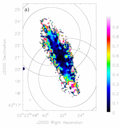
As an example, Fig. 1 (panel a) shows a map of the absolute pixel-by-pixel difference between the PB-corrected spectral index measurements in the two C-band pointings of NGC 891. An increase of the differences with distance from the map centre is clearly apparent. We formed the spectral index error (shown in panel b) by computing the PB-weighted deviation from the average spectral index of the two pointings 9.
 |
 |
 |
 |
Figure 1. a) Absolute difference between the PB-corrected spectral index measurements in the two C-band pointings of NGC 891. There is an increase in difference with distance from the midpoint between the pointing centres, even in regions with high S/N. b) Error of the PB-weighted average of the PB-corrected spectral index measurements in the two pointings. The red contour is placed at an error of 0.1. c) Spectral index error map determined by the ms-mfs clean algorithm (same as panel (k) of the appendix figure of NGC 891, but without the cutoff at Δα > 1.0). Contours represent an error of 0.1 in this map (white) and in the map shown in panel b) (red). d) Ratio of the two different error maps (panel b) divided by panel c)). The ratio is mostly close to unity, except for those parts of the disk lying outside the 0.7 PB level of either pointing. In each panel, the two PB circular contours for each pointing are placed at the 0.5 and 0.7 level. |
|
This error map is for the most part comparable to the error calculated by the ms-mfs algorithm (panel c)), as the map of the ratio of these two errors (panel d)) illustrates. A major exception to this is the disk of the galaxy, but only in those parts that are located outside the 70% PB level (i.e. where the PB gain is less than 0.7) of either pointing. The average error ratio in these narrow regions around the mid-plane is ∼ 5 (with individual pixel values up to ∼ 15), i.e. here the error originating from the pointing differences is on average ∼ 400% higher than the error resulting from the ms-mfs spectral fitting (for comparison, the average error ratio of NGC 4565 is 3.3). Such high ratios are primarily a consequence of the small ms-mfs-based errors in regions of high signal-to-noise, yet the increase of the pointing differences with distance from the pointing centres is significant. In particular, beyond the half-power point the mid-plane errors in panel b) of Fig. 1 increase up to ∼ 0.5, whereas in panel c) they remain below 0.1 throughout the disk, as shown by the displayed contours. While the errors in panel b) are in rough agreement with Bhatnagar et al. (2013) in the sense that they do not exceed 0.1 out to approximately the half-power point (not considering the above-mentioned edge effects), the error ratio map suggests that the simple PB model used by the widebandpbcor task already shows significant inaccuracies at the 70% level.
Resolved out structures:
Although the method of calculating the spectral index ensures that the resolution is common across the band, if there are structures that are resolved out at one end of the band compared to the other, this is not accounted for in the spectral index maps. For example, there may be structures resolved out at the high frequency end of the band, but not at the low frequency end, which would steepen the spectral index.
Comparison with Classical Spectral Index:
A comparison was made between the in-band spectral index and a classically formed spectral index from a given band. The classically formed α maps were made from the spectral index maps after the PB-correction was applied but not after applying further processing (i.e. PB-correction and a 5σ cutoff were applied, but not a cutoff based on the error map, nor smoothing to the size of the beam, as described in Section 3.4.2); they were formed by imaging the lowest end of the band and the highest end of the band, smoothing to a common spatial resolution and then combining in the classical way. The results were in agreement within errors.
Two-pointing PB cutoffs: For ‘two-pointing’ galaxies (large galaxies at C-band) the maps, as indicated in Section 3.3.5, were combined over regions in which the value of the primary beam exceeded 0.1 (10% of the peak). When mosaicking is carried out, each point is weighted by the PB such that points that are farther from the beam centre are weighted down and therefore the difference in total intensity maps, whether one cuts off points where the PB is > 10% or where the PB is > 50%, is entirely negligible. However, since α maps are known to increase quite strongly below the 50% level, we remade our mosaicked α maps with a 50% cutoff to compare it to the 10% cut-off values used in this paper. For these results, we found only minor differences (for example, if the two maps are subtracted, the rms in the regions between the 50% and 10% PB cutoffs is < 0.1).
In summary, our final α maps should present realistic results with the following cautions:
a) Extreme values around the edges are artifacts and should be ignored.
b) Measurements of α should not be quoted ‘per
pixel’ but rather averaged over a beam when carrying out
evaluations or comparisons.
c) The calculated Δα maps typically underestimate the
true errors by ≈ 20% for galaxies of small
angular size
10.
d) The largest source of uncertainty in Δα relates to the
PB model correction away from the pointing centre, which most strongly
affects our largest galaxies in C-band. Spectral index errors increase
significantly with distance from the pointing centre, such that beyond
the 70% PB level of either pointing (i.e. at distances greater than 2'
25"
from the respective pointing centre at C-band) the Δα maps
typically underestimate the true errors in the disk by a factor
∼5 (see Fig 1).
2 For an example of a different weighting, see Paper II for which a naturally weighted map of NGC 4631 was included. Back.
3 Note that the maps shown in panels (e) and (f) of the images in the appendix are the noise biased maps. Peak polarization values have however been measured from the corrected maps. Back.
4 The software is not yet available in CASA. Back.
5 See Eqn. 39 of Rau & Cornwell (2011). Back.
6 For an example showing a result when more than one band is used, see Paper III. Back.
7 The CASA task imsmooth is used. Back.
8 Recently, it has become possible to correct for narrow-band time-varying PB effects during the imaging process using the ‘A-Projection’ algorithm (Bhatnagar et al. 2008, Bhatnagar et al. 2013). However, an algorithm applicable to CHANG-ES data (i.e. for wide bands) is not yet available or practical. Back.
9 √(w1(α1 − αavg)2 + w2(α2 − αavg)2) / (w1 + w2), where w1 = beam1 / beam2 and w2 = beam2 / beam1 Back.
10 Estimated from results where galaxies have been observed in two separate observations. Back.