


There are two major methods to measure the mass distribution using rotation curves, which are the direct method and the decomposition method. In the direct method, the rotation velocity is used to directly calculate the mass distribution. In the decomposition method, a galaxy is represented by superposition of several mass components, and the rotation curve is fitted by searching for the best-fitting parameters of the components.
4.1. Direct Mass Determination
By this direct method the mass distribution in a galaxy is calculated directly from the rotation curve. No functional form is necessary to be given a priori. Only an assumption has to be made, either if the galaxy's shape is a sphere or a flat disk. The 'true' mass profile is considered to lie between the two extreme cases of the spherical and axisymmetric disk distribution.
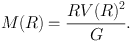
On the assumption of spherical distribution, the mass inside radius R is given by
 |
(34) |
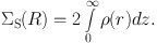
Then the surface-mass density (SMD) ΣS(R) at R is calculated by
 |
(35) |
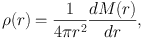
Remembering
 |
(36) |
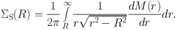
the above expression can be rewritten as
 |
(37) |
This gives good approximation for spheroidal component in the central region, but results in underestimated mass in the outer regions. Particularly, the approximation fails in the outermost region near the end of rotation curve due to the edging effect of integration.
The SMD of a flat thin disk, ΣD(R), is calculated by solving the Poisson's equation on the assumption that the mass is as symmetrically distributed in a disk of negligible thickness (Freeman 1970; Binney and Tremaine 1987). It is given by
 |
|
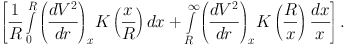 |
(38) |
Here, K is the complete elliptic integral, which becomes very large when x ≃ R.
A central black hole may influence the region within ∼ 1, but it does not affect much the galactic scale SMD at lower resolution. Since it happens that there exist only a few data points in the innermost region, the reliability is lower than the outer region. Since the rotation curves are nearly flat or declining outward beyond maximum, the SMD values are usually slightly overestimated in the outer disk.
4.1.3. Milky Way's direct mass calculation
Figure 21 shows SMD distributions in the Galaxy calculated by the direct methods for the sphere and flat-disk cases, compared with SMD calculated for the components obtained by deconvolution of the rotation curve. There is remarkable similarity between the results by direct methods, and by RC deconvolution.
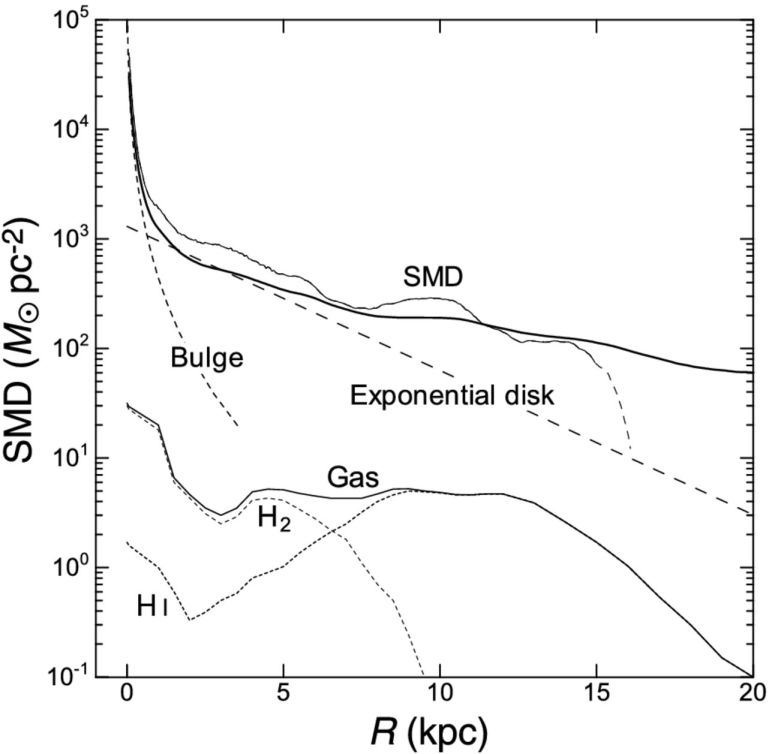 |
Figure 21. SMD distribution in the Milky Way. Thick line shows the directly calculated SMD for thin disk case, and thin line shows result for spherical case. The long dashed smooth lines are model profile for de Vaucouleurs and exponential disk. The lower lines show SMD of interstellar gas made by annulus-averaging of figure 7 (Nakanishi and Sofue 2003, 2006, 2016). HI and H2 gas SMDs are also shown separately by dotted lines. (Bottom) Same, but for spiral galaxies. |
The SMD is strongly concentrated toward the center, reaching SMD as high as ∼ 105 M⊙ pc2 within ∼ 10 pc. The galactic disk appears as an exponential disk as indicated by the straight-line at R ∼ 3 to 8 kpc on the semi-logarithmic plot. It is worth to note that the dynamical SMD is dominated by dark matter, because the SMD is the projection of extended dark halo. Note, however, that the volume density in the solar vicinity is dominated by disk's stellar mass. The outer disk is followed by an outskirt with a slowly declining SMD profile, which indicates the dark halo and extends to the end of the rotation curve measurement.
In figure 21, we also show the radial distribution of interstellar gas density, as calculated by azimuthally averaging the gas density distribution in figure 7. The gas density is much smaller than the dynamical mass density by an order of magnitude. The SMD of ISM is ∼ 5.0 M⊙ pc−2 R ∼ 8 kpc, sharing only several percents of disk mass density ∼ 87.5 M⊙ pc−2.
The SMDs obtained by deconvolution and direct methods are consistent with each other within a factor of ∼ 1.5. At R ∼ 8 kpc, the directly calculated SMD is ∼ 300 M⊙ pc−2, whereas it is ∼ 200−250 M⊙ pc−2 by deconvolution, as shown in figure 22.
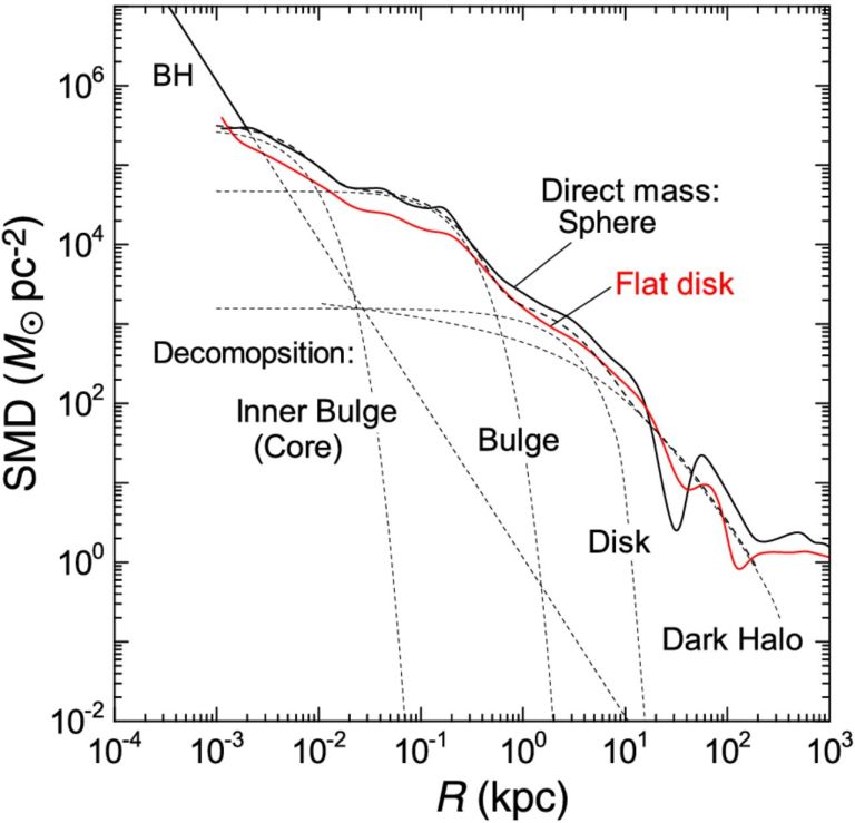 |
Figure 22. Directly calculated SMD of the Milky Way by spherical (black thick line) and flat-disk assumptions by log-log plot, compared with the result by deconvolution method (dashed lines). The straight line represents the black hole with mass 3.6 × 10⁶ M⊙. |
4.1.4. Spiral galaxies' direct mass
Figure 23 shows SMD distributions of spiral galaxies calculated for the rotation curves shown in figure 14 using the direct methods. Results for flat-disk assumption give stable profiles in the entire galaxy, while the sphere assumption yields often unstable mass profile due to the edge effect in the outermost regions. On the other hand, the central regions are better represented by the sphere assumption because of the suspected spherical distribution of mass inside the bulge.
 |
Figure 23. (a) Direct SMD in spiral galaxies with end radii of RC greater than 15 kpc (from Sofue 2016) calculated under flat disk assumption, and the same in logarithmic radius (Sofue 2016). Red dashed lines indicates the Milky Way. (b) Same but under sphere assumption. |
The calculated SMD profiles for galaxies are similar to that of the Milky Way. Namely, dynamical structures represented by the density profiles in spiral galaxies are similar to each other, exhibiting universal characteristics as shown in the figures: high central concentration, exponential disk, and outskirt due to the dark halo.
4.1.5. Mass-to-luminosity ratio
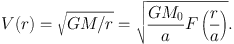
The farthest rotation velocity so far measured for a spiral galaxy is that for the Milky Way and M31 up to ∼ 300 kpc, where the kinematics of satellite galaxies was used to estimate the circular velocities (Sofue 2012, 2013b). The obtained rotation curve was shown to be fitted by the NFW density profile.
Note, however, that the NFW model predicts declining rotation only beyond galacto-centric distances farther than ∼ 50 kpc. Inside this radius, there is not much difference in the RC shapes of NFW model and isothermal model, predicting almost flat (NFW) or perfectly flat (isothermal) rotation. Practically for most galaxies with rotation curves up to ∼ 30 kpc, both the models yield about the same result about their halos. In either models, observed rotation velocities in spiral galaxies show that the mass in their halos is dominated by dark matter.
The mass-to-luminosity (M/L) ratio can be obtained by dividing SMD by surface luminosity profiles (Forbes 1992; Takamiya and Sofue 2000; Vogt et al. 2004a). Figure 24 shows M/L ratios for various spiral galaxies normalized at their scale radii (Takamiya and Sofue 2000). While the M/L ratio is highly variable inside their disk radii, it increases monotonically toward galaxies' edges. However, the outermost halos farther than ∼ 20−30 kpc, beyond the plotted radii in the figure, the M/L ratio is extremely difficult to determine from observations because of the limited finite radii of the luminous disks, beyond which the surface brightness is negligibly low, and hence the M/L ratio tends to increase to infinity.
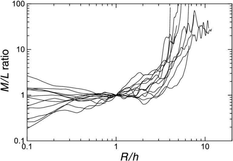 |
Figure 24. M/L ratios in spiral galaxies normalized at scale radii using data from Takamiya and Sofue (1999), where L is the optical luminosity. |
4.2. Rotation Curve Decomposition into Mass Components
4.2.1. Superposition of mass components
The rotation velocity is written by the gravitational potential as
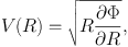 |
(39) |
where
 |
(40) |
with Φi being the potential of the i-th mass component. Knowing that Vi(R) = R ∂ Φi / ∂ R, we have
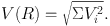 |
(41) |
It is often assumed that there are multiple components that are the central black hole, a bulge, disk and a dark halo:
 |
(42) |
Here, the suffice BH represent black hole, b for bulge, d for disk and h for the dark halo.
The parameters (masses and scale radii of individual components) are iteratively determined by the least χ2 fitting (Carignan 1985; Carignan and Freeman 1985). First, an approximate set of the parameters are given as an initial condition, where the values of the parameters are hinted by luminosity profiles of the bulge and disk, and by the shape and amplitude of the rotation curve for the dark halo. All the parameters are fitted at once to fit the observed rotation curve.
When precise rotation curves are available with a larger number of data points, particularly in the resolved innermost regions of the Milky Way and nearby galaxies, the fitting may be divided into several steps according to the components in order to save the computation time (Sofue 2012). The time per one iteration is proportional to nN, where n is the number of data points and N is the number of combination of parameters. The combination number is given by N = (Σi ni)!, where ni is the number of parameters of the i-th component. On the other hand, it is largely reduced to N = Σi (ni !) in the step-by-step method.
Also, it is useful to divide the fitting radii depending on the component's properties. Namely, a black hole and bulge may not be fitted to data beyond the disk, e.g., beyond R ∼ 10 kpc, while a halo may not be fitted at < ∼ 1 kpc. This procedure can save not only the time, but also the degeneracy problem (Bershady et al. 2010a, b). Degeneracy happens for data with low resolution and small number of measurements, often in old data, in such a way that a rotation curve is represented equally by any of the mass models, or, the data is fitted either by a single huge bulge or disk, or by a single tiny halo.
In the step-by-step method, a set of the parameters are assumed, first, as the initial condition as above. The fitting is started individually from the innermost component having the steepest rise (gradient), which is particularly necessary when a black hole is included. Next, the steeply rising part by the bulge is fitted, and then gradual rise and flat parts are fitted by the disk. Finally, the residual outskirt is fitted by a dark halo. This procedure is repeated iteratively, starting again from the innermost part, until the χ2 value is minimized.
Observed rotation curves in spiral galaxies may be usually fitted by three components of the bulge, disk and dark halo. In the Milky Way, the rotation curve may better be represented by four or five components which are the central black hole, multiple bulges, an exponential disk, and dark halo.
 |
Figure 25. (a) Analytic rotation curve composed of bulge, disk and dark halo components represented by isothermal, Burkert (1995) and NFW models (full lines from top to bottom at R = 30 kpc). Dashed lines represent de Vaucouleurs bulge and exponential disk. (b) Corresponding volume densities. (c) Corresponding enclosed mass within radius r. |
The Galactic Center of the Milky Way is known to nest a massive black hole of mass of MBH = 2.6−4.4 × 10⁶ M⊙ (Genzel et al. 1994, 1997, 2000, 2010), 4.1−4.3 × 10⁶ M⊙ (Ghez et al. 1998, 2005, 2008), and 3.95 × 10⁶ M⊙ (Gillessen et al. 2009).
A more massive black hole has been observed in the nucleus of the spiral galaxy NGC 4258 with the mass of 3.9 × 10⁷ M⊙ (Nakai et al. 1993; Miyoshi et al. 1995; Herrnstein et al. 1999) from VLBI observations of the water maser lines. Some active galaxies have been revealed of rapidly rotating nuclear torus of sub parsec scales indicating massive black holes in several nearby active galactic nuclei, and increasing number of evidences for massive black holes in galactic nuclei have been reported (Melia 2010). Statistics shows that the mass (luminosity) of bulge is positively related to the mass of central black hole (Kormendy and Westpfahl 1989; Kormendy 2001).
The most commonly used profile to represent the central bulge is the de Vaucouleurs (1958) law (figure 26), which was originally expressed by a surface-brightness distribution at projected radius R by
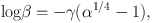 |
(43) |
where γ = 3.3308. Here, β = Bb(R) / Bbe, α = R / Rb , and Bb(R) is the surface-brightness normalized by the value at radius Rb, Bbe.
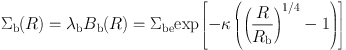
The same de Vaucouleurs profile for the surface mass density is usually adopted for the surface mass density as
 |
(44) |
with Σbc = 2142.0 Σbe for κ = γ ln 10 = 7.6695. Here, λb is the M/L ratio assumed to be constant.
Equations (43) and (44) show that the central SMD at R = 0 attains a finite value, and the SMD decreases steeply outward near the center. However, the decreasing rate gets much milder at large radii, and the SMD decreases slowly, forming an extended outskirt (de Vaucouleurs 1958).
The cylindrical mass inside R is calculated
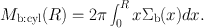 |
(45) |
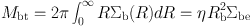
Total mass of the bulge given by
 |
(46) |
with η = 22.665. A half of the total projected (cylindrical) mass is equal to that inside a cylinder of radius Rb.
The volume mass density ρ(r) at radius r for a spherical bulge is now given by
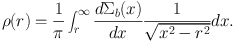 |
(47) |
The circular velocity is thus given by the Kepler velocity of the mass inside R as
 |
(48) |
where
 |
(49) |
Note that the spherical mass Mb:sph(R) is smaller than the cylindrical mass Mb:cyl(R) given by equation (45). At large radii, the velocity approximately decreases by Keplerian-law. Figure 26) shows the variation of circular velocity for a de Vaucouleurs bulge.
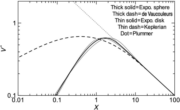 |
Figure 26. Comparison of normalized rotation curves for the exponential spheroid, de Vaucouleurs spheroid, and other typical models, for a fixed total mass. The exponential spheroid model is almost identical to that for Plummer law model. The central rise of de Vaucouleurs curve is proportional to ∝ r1/2, while the other models show central velocity rise as ∝ r. |
The de Vaucouleurs law has been extensively applied to fit spheroidal components of late type galaxies (Noordermeer 2007, 2008). Sérsic (1958) has modified the law to a more general form e−(R / re)n. The de Vaucouleurs and Sérsic laws were fully discussed in relation to its dynamical relation to the galactic structure based on the more general profile (Ciotti 1991; Trujillo 2002). The de Vaucouleurs law has been also applied to fit the central rotation curve of the Milky Way as shown in figure 4. However, it was found that the de Vaucouleurs law cannot reproduce the observations inside ∼ 200 pc.
It is interesting to see the detailed behavior of the de Vaucouleurs law. At the center, Σ reaches a constant, and volume density varies as ∝ 1/r, leading to circular velocity V ∝ r1/2 near the center. Thus, the rotation velocity rises very steeply with infinite gradient at the center. It should be compared with the mildly rising velocity as V ∝ r in the other models. Figure 26 compares normalized behaviors of rotation velocity for de Vaucouleurs and other models.
The de Vaucouleurs rotation curve shows a much broader maximum in logarithmic plot compared to the other models, because the circular velocity rises as V ∝ √M(< r) / r ∼ √r. The particular behavior can be better recognized by comparing the half-maximum logarithmic velocity width with other models, where the width is defined by
 |
(50) |
Here, r2 and r1 (r2 > r1) are the radii at which the rotational velocity becomes half of the maximum velocity. From the figure, we obtain Δlog = 3.0 for de Vaucouleurs , while Δlog = 1.5 for the other models as described later. Thus the de Vaucouleurs's logarithmic curve width is twice the others, and the curve's shape is much milder.
Since it was shown that the de Vaucouleurs law fails to fit the observed central rotation, another model has been proposed, called the exponential sphere model. In this model, the volume mass density ρ is represented by an exponential function of radius r with a scale radius a as
 |
(51) |
The mass involved within radius r is given by
 |
(52) |
where x = r / a and
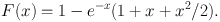 |
(53) |
The total mass is given by
 |
(54) |
The circular rotation velocity is then calculated by
 |
(55) |
In this model the rotational velocity has narrower peak near the characteristic radius in logarithmic plot as shown in figure 26. Note that the exponential-sphere model is nearly identical to that for the Plummer's law, and the rotation curves have almost identical profiles. In this context, the Plummer law can be used to fit the central bulge components in place of the present models.
The galactic disk is represented by an exponential disk (Freeman 1970), where the surface mass density is expressed as
 |
(56) |
Here, Σdc is the central value, Rd is the scale radius. The total mass of the exponential disk is given by Mdisk = 2 π Σdc Rd2. The rotation curve for a thin exponential disk is expressed by (Binney and Tremaine 1987).
 |
|
 |
(57) |
where y = R / (2Rd , and Ii and Ki are the modified Bessel functions.
If the surface mass density does not obey the exponential law, the gravitational force f(R) can be calculated by integrating the x directional force caused by mass element Σd′ (x) dx dy in the Cartesian coordinates (x, y):
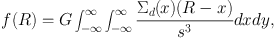 |
(58) |
where s = √(R − x)2 + y2 . The rotation velocity is then given by
 |
(59) |
This formula can be used for any thin disk with an arbitrary SMD distribution Σ(x, y), even if it includes non-axisymmetric structures.
4.2.6. Isothermal and NFW dark halos
4.2.6.1. Evidence for dark matter halo
The existence of dark halos in spiral galaxies has been firmly evidenced from the well established difference between the galaxy mass predicted by the luminosity and the mass predicted by the rotation velocities (Rubin et al. 1980-1985; Bosma 1981a, b; Kent 1986, 1987; Persic and Salucci 1990; Salucci and Frenk 1989; Forbes 1992; Persic et al. 1996; Héraudeau and Simien 1997; Takamiya and Sofue 2000).
In the Milky Way, extensive analyses of motions of non-disk objects such as globular clusters and dwarf galaxies in the Local Group have shown flat rotation up to ∼ 100 kpc, and then declining rotation up to ∼ 300 kpc (Sofue 2013, 2015). The outer rotation velocities have made it to analyze the extended distribution of massive dark halo, which is found to fill the significantly wide space in the Local Group. Bhattacharjee et al. (2013, 2014) have analyzed non-disk tracer objects to derive the outer rotation curve up to 200 kpc in order to constrain the dark matter mass of the Galaxy, reaching a consistent result. As will be shown later, the dark halos of the Milky Way and M31 are shown to be better represented by the NFW model than by isothermal halo model.
The simplest model for the flat rotation curve is the semi-isothermal spherical distribution (Kent 1986; Begeman et al. 1991), where the density is written as
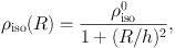 |
(60) |
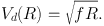
where ρiso and h = Rh are the central mass density and scale radius, respectively. The circular velocity is given by
 |
(61) |
which approaches a constant rotation velocity V∞ at large distances. At small radius, R≪ h, the density becomes nearly constant equal to ρiso0 and the enclosed mass increases steeply as M(R) ∝ R3. At large radii, the density decreases with ρiso ∝ R−2. The enclosed mass increases almost linearly with radius as M(R) ∝ R.
4.2.6.3. Navarro-Frenk-White (NFW) model
The most popular model for the dark halo is the NFW model (Navarro, Frenk and White 1996, 1997) empirically obtained from numerical simulations in the cold-dark matter scenario of galaxy formation. Burkert's (1995) modified model is also used when the singularity at the nucleus is to be avoided. The NFW density profile is written as
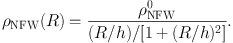 |
(62) |
The circular velocity is equal to
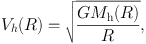 |
(63) |
where Mh is the enclosed mass within the scale radius h.
At R ≪ h, the NFW density profile behaves as ρNFW ∝ 1/R, yielding an infinitely increasing density toward the center, and the enclosed mass behaves as M(R) ∝ R2. The Burkert's modified profile tends to constant density ρBur0, similar to the isothermal profile.
At large radius the NFW shows density profile as ρNFW, Bur ∝ R−3, yielding logarithmic increasing of mass, M(R) ∝ ln R (Fig. 25 ). Figure 25 shows density distributions for the isothermal, NFW and Burkert models.
4.2.7. Plummer and Miyamoto-Nagai potential
The current mass models described above do not necessarily satisfy the Poisson's equation, and hence, they are not self consistent for representing a dynamically relaxed self-gravitating system. In order to avoid this inconvenience, Plummer-type potentials are often employed to represent the mass distribution.
The Miyamoto and Nagai's (MN) (1975) potential is one of the most convenient Plummer-type formulae to describe a disk galaxy's potential and mass distribution in an analytic form:
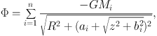 |
(64) |
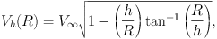
where, Mi, ai and bi are the mass, scale radius and height of the i-th spheroidal component. The rotation velocity in the galactic plane at z = 0 is given by
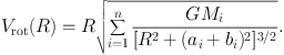 |
(65) |
The mass distribution is given by the Poisson's equation:
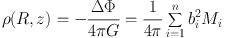 |
|
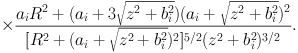 |
(66) |
This model was used to approximate the observed rotation curve of the Milky Way (Miyamoto and Nagai 1975). Their proposed parameters are often used to represent a bulge and disk for numerical simulations not only in the original form, but also by adding a larger number of components by choosing properly the masses and scale radii. The original parameters were given to be Mbulge ∼ 2.05 × 10¹⁰ M⊙, abulge = 0, bbulge ∼ 0.495 kpc, and Mdisk ∼ 2.547 × 10¹¹ M⊙, adisk ∼ 7.258 pc, bdisk ∼ 0.520 kpc.
The models described here are expressed by single-valued simple analytic functions. Each of the functions has only two parameters (mass and size). The black hole is expressed by the Keplerian law with only one parameter (mass). The mass and scale radius of the de Vaucouleurs law are uniquely determined, if there are two measurements of velocities at two different radii, and so for the exponential disk and NFW halo.
If the errors are sufficiently small, the three major components (bulge, disk and halo) can be uniquely determined by observing six velocity values at six different radii. In actual observations, the number of data points are much larger, while the data include measurement errors. Hence, the parameters are determined by statistically by applying the least-squares fitting method or the least χ2 method. Thereby, the most likely sets of the parameters are chosen as the decomposition result.
However, when the errors are large and the number of observed points are small, degeneracy problem becomes serious (Bershady et al. 2010a, b), where the fitting is not unique. Such a peculiar case sometimes happens, when the rotation curve is mildly rising and tends to flat end, that the curves fitted in almost the same statistical significance either by a disk and halo, by a single disk, or by a single halo. Such mild rise of central rotation is usually observed in low-resolution measurements.
4.3. Rotation Curve Decomposition in the Milky Way
Observed mass components in the Galaxy and spiral galaxies are often expressed by empirical functions derived by surface photometry of the well established bulge and disk. Also, central black hole and outermost dark halo are the unavoidable components to describe resolved galactic structures.
4.3.1. Black hole, bulge, disk and halo of the Milky Way
In the rotation curve decomposition in the Milky Way, the following components have been assumed (Sofue 2013):
An initially given approximate parameters were adjusted to lead to the best-fitting values using the least χ2 method. Figure 4 shows the fitted rotation curve, which satisfactorily represents the entire rotation curve from the central black hole to the outer dark halo. Figures 27 and 28 show the variation of ?2 values around the best-fitting parameters.
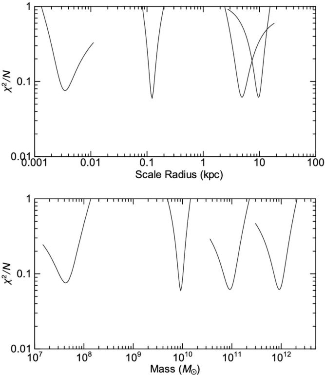 |
Figure 27. χ2 plots around the best-fit values of the scale radii of the deconvolution components to obtain figure 4. |
 |
Figure 28. Contour presentation of two dimensional distribution of log χ2 value around the best-fit points in the scale radius-mass space to obtain figure 4. |
The fitting of the two peaks of rotation curve at r∼ 0.01 kpc and ∼ 0.5 kpc are well reproduced by the two exponential spheroids. The figure also demonstrates that the exponential bulge model is better than the de Vaucouleurs model. It must be mentioned that the well known de Vaucouleurs profile cannot fit the Milky Way's bulge, while it is still a good function for fitting the bulges in extragalactic systems. Table 6 lists the fitting parameters for the Milky Way.
| Mass component | Quantities |
| Black hole | Mbh = 3.6 × 10⁶ M⊙‡ |
| Bulge 1 (massive core) | ab = 3.5 ± 0.4 pc |
| Mb = 0.4 ± 0.1 × 10⁸ M⊙ | |
| Bulge 2 (main bulge)* | ab = 120 ± 3 pc |
| Mb = 0.92 ± 0.02× 10¹⁰ M⊙ | |
| Disk | ad = 4.9 ± 0.4 kpc |
| Md = 0.9 ± 0.1 × 10¹¹ M⊙ | |
| Dark halo | h = 10 ± 0.5 kpc |
| ρ0 = 2.9 ± 0.3 × 10⁻² M⊙ pc−3 | |
| MR < 200 kpc = 0.7 ± 0.1 × 10¹² M⊙ | |
| MR < 385 kpc = 0.9 ± 0.2 × 10¹² M⊙ | |
| DM density at Sun | ρ8 = 0.011 ± 0.001 M⊙ pc−3 |
| = 0.40 ± 0.04 GeV cm−3 | |
| † The adopted galactic constants are (R0, V0) = (8 kpc, 238 km s−1) (Honma et al 2012). | |
| ‡ Genzel et al. (2000 - 2010) | |
| * Mb is the surface mass enclosed in a cylinder of radius ab, but not a spherical mass. | |
Figure 29 shows the enclosed mass in the Galactic Center as a function of radius calculated for the parameters obtained by rotation curve decomposition. The plots are compared with the measured values at various radii, as compiled by Genzel et al. (1994), where their data have been normalized to R0 = 8.0 kpc. It should be stressed that both the plots are in good agreement with each other. The figure shows that the bulge density near the center tends to constant, so that the innermost enclosed mass behaves as ∝ r3 as the straight part of the plot indicates. On the other hand, the disk has a constant surface density near the center, and hence the enclosed mass varies as ∝ r2, as the straight line for the disk indicates. The NFW model predicts a high density cusp near the center with enclosed surface mass ∝ r2, as shown by the dashed line, exhibiting similar behavior to the disk.
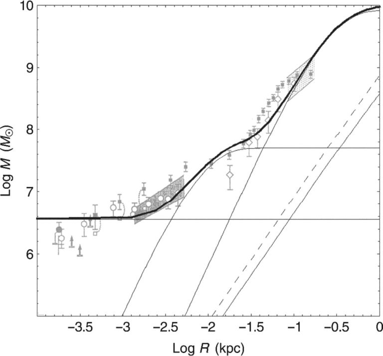 |
Figure 29. Enclosed mass calculated for the Galaxy's rotation curve compared to those by Genzel et al. (1994). The horizontal line, thin lines, and dashed line indicate the black hole, inner bulge, main bulge, disk, and dark matter cusp. |
4.3.3. Local dynamical values and dark matter density
The local value of the volume density of the disk can be calculated by ρd = Σd / (2 z0), where z0 is the vertical scale height at radius R = R0, when the disk scale profile is approximated by ρd(R0, z) = ρd0(R0) sech (z / z0). The disk thickness has been observed to be z0 = 144 ± 10 pc for late type stars using the HYPPARCOSS catalogue (Kong and Zhu 2008), while a larger value of 247 pc is often quoted as a traditional value (Kent et al. 1991).
The local volume density by the bulge and dark halo is ∼ 10−4 and ∼ 10−2 times the disk density, respectively. However, the SMD projected on the Galactic plane of the bulge contributes to 1.6% of the disk value. It is interesting to note that the SMD of the dark halo exceeds the SMD of the disk by several times.
The NFW model was found to fit the grand rotation curve quite well (Sofue 2012), including the declining part in the outermost rotation at R ∼ 40−400 kpc. The local dark matter density is a key quantity in laboratory experiments for direct detection of the dark matter. Using the best fit parameters for the NFW model, the local dark matter density in the Solar neighborhood is calculated to be ρ0⊙ = 0.235 ± 0.030 GeV cm−3. This value may be compared with the values obtained by the other authors as listed in table 7.
| Author | ρs (GeV cm−3) |
| Weber and de Boer (2010) | 0.2 - 0.4 |
| Salucci et al. (2012) | 0.43 ± 0.10 |
| Bovy and Tremaine (2012) | 0.3 ± 0.1 |
| Piffl et al. (2014) | 0.58 |
| Sofue (2013b), V0 = 200 km s-1 | 0.24± 0.03 |
| —–, V0 = 238 km s-1 | 0.40 ± 0.04 |
| Pato et al (2015a, b), V0 = 230 km s-1 | |
4.4. Decomposition of Galaxies' Rotation Curves
4.4.1. Bulge, disk and NFW halo decomposition of spiral galaxies
The mass decomposition has been also applied extensively to spiral galaxies with relatively accurate rotation curves. It is a powerful tool to study the relations among the scale radii and masses of the bulge and disk with those of the dark halo, which provides important information about the structure formation in the universe (Reyes et al. 2012; Miller et al. 2014; Behroozi et al. 2013).
Decomposition has been applied to galaxies as compiled in figure 14 (Sofue 2016) by adopting the de Vaucouleurs , exponential and NFW density profiles for the bulge, disk and dark halo, respectively. The best-fitting values were obtained by applying the least χ2 method for Mb, ab, Md, ad, ρ0 and h. The critical dark halo radius, R200, critical mass, M200, as well as the mass, Mh, enclosed within the scale radius h were also calculated, which are defined by
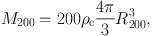 |
(67) |
and
 |
(68) |
with H0 = 72 km s−1 Mpc−1 being the Hubble constant.
Figure 30 shows examples of rotation curves and fitting result for NGC 891. The figure also shows the variation of χ2 values plotted against the parameters. Applying a selection criterion, the fitting was obtained for 43 galaxies among the compiled samples in figure 14, and the mean values of the results are shown in table 8.
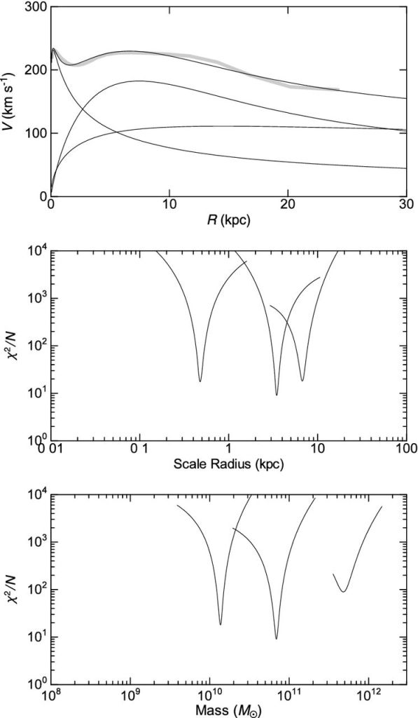 |
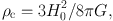
Figure 30. Rotation curve and χ2 fitting result for NGC 891 (top), distribution of χ2 / N around the best fit scale radii (middle) and masses (bottom) of the three components. |
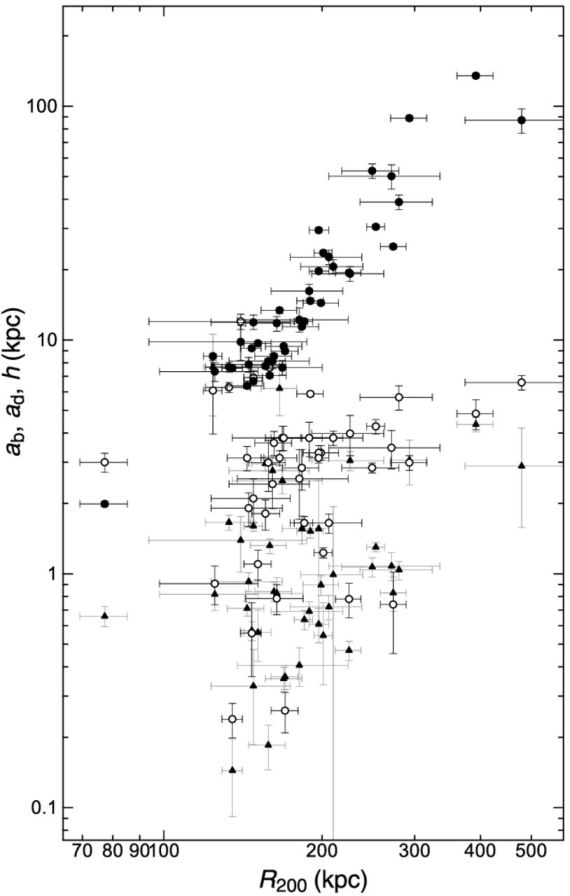 |
Figure 31. Size-Size relations for dark halo critical radius for (R200, ab) (triangles); R200, ad) (open circles); and (R200, h) (black dots) (Sofue 2016) |
| Bulge size | ab | 1.5 ± 0.2 kpc |
| — mass | Mb | 2.3 ± 0.4 1010 M⊙ |
| Disk size | ad | 3.3 ± 0.3 kpc |
| — mass | Md | 5.7 ± 1.1 × 10¹⁰ M⊙ |
| DH scale size | h | 21.6 ± 3.9 kpc |
| —mass within h | Mh | 22.3 ± 7.3 × 10¹⁰ M⊙ |
| —critical radius | R200 | 193.7 ± 10.8 kpc |
| —critical mass | M200 | 127.6 ± 32.0 × 10¹⁰ M⊙ |
| Bulge+Disk | Mb+d | 7.9 ± 1.2 × 10¹⁰ M⊙ |
| Bulge+Disk+Halo | MTotal† | 135.6 ± 32.0 × 10¹⁰ M⊙ |
| B+D / Halo ratio | Mb+d / M200 | 0.062 ± 0.018 |
| B+D / Total ratio | Mb+d / MTotal | 0.059 ± 0.016 |
| † MTotal = M200+b+d | ||
4.4.2. Size and mass fundamental relations
Correlations among the deconvolved parameters are useful to investigate the fundamental relations of dynamical properties of the mass components (e.g., Vogt et al. 2004a, b). Figure 32 shows plots of ab, ad, and h against the critical radius R200 for the compiled nearby galaxies (Sofue 2015). It is shown that the bulge, disk and halo scale radii are positively correlated with R200. Note that the tight correlation between h and R200 includes the trivial internal relation due to the definition of the two parameters connected by ρ0 through equation (67).
 |
Figure 32. Size-Mass relations for (R200, Mb) (triangles); (R200, Md) (rectangles); (R200, Mh) (black dots); (R200, M200) (grey small dots) showing the trivial relation by definition of the critical mass. |
The figure also shows Mb+d plotted against M200, which may be compared with the relation of stellar masses of galaxies against dark halo masses as obtained by cosmological simulation of star formation and hierarchical structure formation by Behroozi et al. (2013). The grey dashed line shows the result of simulation at z = 0.1.
Figure 33 shows the bulge+disk mass, Mb+d, plotted against total mass, M200+b+d = M200+Mb+d. In the figure we also plot photometric luminous mass and Virial mass obtained for dwarf galaxies by Miller et al. (2014). Also compared is a cosmological simulation by Behroozi et al. (2013). The simulation is in agreement in its shape with the plots for spiral and dwarf galaxies. The shape of simulated relation is consistent with the present dynamical observations, while the absolute values of Mb+d are greater than the simulated values by a factor of three. Solving the discrepancy may refine the cosmological models and will be a subject for the future.
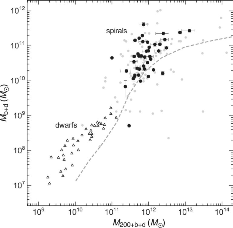 |
Figure 33. Mb+d - M200+b+d relation compared with the stellar mass-total mass relation for dwarf galaxies (triangle: Miller et al. 2014) and simulation + photometry (grey dashed line: Behroozi et al. 2013). Black dots are the selected galaxies with reasonable fitting results, while small grey dots (including black dots) show non-weighted results from automatic decomposition of all rotation curves. |
The obtained correlations between the size and mass are the dynamical manifestation of the well established luminosity-size relation by optical and infrared photometry (de Jong et al. 1999; Graham and Worley 2008; Simard et al. 2011). It is interesting to notice that a similar size-mass relation is found for dark halos.
The size-mass correlations can be fitted by straight lines on the log-log planes using the least-squares fitting. Measuring the mass and scale radii in M⊙ and kpc, respectively, we have size-mass relations for the disk and dark halo as
 |
(69) |
 |
(70) |
However, the relation for the bulge is too diverged to be fitted by a line.
The size-mass relation for the disk agrees with the luminosity-size relation obtained by Simard et al. (2011). It is found that the relations for the disk and dark halo can be represented by a single (common) relation
 |
(71) |
where Mi = Mb+d or M200 in 1010 M⊙ and ai = ad or h in kpc. This simple equation leads to a relation between the bulge+disk mass to halo mass ratio, which approximately represents the baryonic fraction, expressed by the ratio of the scale radii of disk to halo as
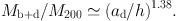 |
(72) |
For the mean values of < ad > = 3.3 kpc and < h > = 21.6 kpc, we obtain Mb+d / M200 ∼ 0.07.