


The basic idea behind the SBF
technique is quite straightforward: the fluctuations in unresolved star
clusters of the Milky Way and other galaxies appear, due to the
Poisson statistics (which is the counting statistics of discrete stars),
to be clumpy and mottled, whereas in more distant objects the fluctuations
appear more smooth. These spatial brightness variations, which are
distance-dependent in amplitude and varying for a given resolution element,
are proportional to
 √N, where
denotes the mean flux
per star and N is the mean number of stars per pixel.
Note that these values are summed over all stars of a stellar system.
The mean intensity per resolution element is
N ; therefore the
difference between the spatial variance and the observed mean results in the
average flux per star ,
which decreases inversely with the square of
the distance d−2.
is the average flux of
the underlying stellar population, weighted to its luminosity, and
corresponds for evolved stellar populations roughly to the flux of a
typical old giant star between spectral type K to M within the
Hertzsprung-Russell diagram. If the mean absolute magnitude
√N, where
denotes the mean flux
per star and N is the mean number of stars per pixel.
Note that these values are summed over all stars of a stellar system.
The mean intensity per resolution element is
N ; therefore the
difference between the spatial variance and the observed mean results in the
average flux per star ,
which decreases inversely with the square of
the distance d−2.
is the average flux of
the underlying stellar population, weighted to its luminosity, and
corresponds for evolved stellar populations roughly to the flux of a
typical old giant star between spectral type K to M within the
Hertzsprung-Russell diagram. If the mean absolute magnitude
 is known, it is possible to determine the distance of the target object.
Inversely, knowing the distance,
can be
established, which
itself yields information on the stellar population of a galaxy.
is known, it is possible to determine the distance of the target object.
Inversely, knowing the distance,
can be
established, which
itself yields information on the stellar population of a galaxy.
The average stellar luminosity
 of a stellar
system (star cluster or galaxy), which is summed over all stars (see
equation 2), is defined as
= 4 π
d2.
is
weighted towards the brightest stars of a specific population.
For the typical old, evolved and metal-rich stellar
populations of elliptical galaxies, these are cool, luminous, Red
Giant Branch (RGB) stars
(3.2 ≲ log(Lbol / L⊙)
≲ 4.2)
and Thermally-Pulsating Asymptotic Giant Branch (TP-AGB) stars.
Since (TP-)RGB stars have a red colour, the SBF magnitudes are red;
ellipticals typically display
of a stellar
system (star cluster or galaxy), which is summed over all stars (see
equation 2), is defined as
= 4 π
d2.
is
weighted towards the brightest stars of a specific population.
For the typical old, evolved and metal-rich stellar
populations of elliptical galaxies, these are cool, luminous, Red
Giant Branch (RGB) stars
(3.2 ≲ log(Lbol / L⊙)
≲ 4.2)
and Thermally-Pulsating Asymptotic Giant Branch (TP-AGB) stars.
Since (TP-)RGB stars have a red colour, the SBF magnitudes are red;
ellipticals typically display
 I
− K
≈ 4.20 ± 0.10
(Jensen et al. 1998).
The preferred photometric bands for SBF observations are
either the red (VRI) or the NIR filter bandpasses
(JHK). NIR filters are preferred over optical wavelength bands,
owing to two advantages in particular: (i) the SBF signal is
dominated by red, luminous giant stars, and (ii) there are
smaller extinction corrections due to lower dust absorption in the
stellar systems. However, the Kron-Cousins I-band supersedes the
NIR-bands because of its relative insensitivity to spatial variations in
the stellar populations.
I
− K
≈ 4.20 ± 0.10
(Jensen et al. 1998).
The preferred photometric bands for SBF observations are
either the red (VRI) or the NIR filter bandpasses
(JHK). NIR filters are preferred over optical wavelength bands,
owing to two advantages in particular: (i) the SBF signal is
dominated by red, luminous giant stars, and (ii) there are
smaller extinction corrections due to lower dust absorption in the
stellar systems. However, the Kron-Cousins I-band supersedes the
NIR-bands because of its relative insensitivity to spatial variations in
the stellar populations.
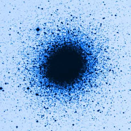 |
Figure 2. A high S / N exposure of the galactic globular cluster M2. The composite ESO/Digitized Sky Survey 2 (DSS2) 1 image clearly shows an obvious strong lumpiness and mottling that is caused by the dominant evolved giant star population. The same mechanism works for other stellar systems, such as galaxies, but is less evident because of their more complex stellar content and greater distance. |
An observational example for the effect of spatial brightness variations
is given in Figure 2. A high S / N
image of the galactic globular cluster
M2 shows very nicely a strong lumpiness and mottling caused by the dominant
evolved giant star population. In principle, this mechanism also works for
galaxies, but for enhancing effects a GC was chosen. In a first step, a
CCD detector measures the total flux per pixel. From this total flux
the average flux per pixel (which is also known as surface brightness)
and the root-mean-square (rms) variation of the flux from pixel-to-pixel
can be derived. However, it is impossible to distinguish the two stellar
systems by their average flux per pixel, because the number of stars
per pixel of a resolution element increases with the distance
d2,
whereas simultaneously the flux per star decreases inversely with the
square of the distance (1 / d2).
Stars cannot be resolved individually; only a characteristic (mean) flux
per pixel can be established. If the number of detected photons within a
resolution element is larger than the projected number of stars within this
area, the fluctuations are proportional to the square root of the number of
stars; i.e., the variations follow
√N, with
being the
average flux per star and N the average number of stars per
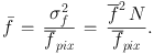
pixel. Thus, the variance of fluctuations
σf2 is derived from the square of the
fluctuations from pixel-to-pixel as σf2
= 2 N,
where N denotes
the mean flux per pixel. The average flux per star is determined from
the ratio between the fluctuation variance and the average flux per pixel as
 |
(1) |
is the average flux of
the underlying stellar population, weighted to
its luminosity, and corresponds for evolved stellar populations
roughly to the flux of old RGB stars.
A sketch of the SBF technique is illustrated in
Figure 3.
Let us compare two stellar systems, a nearby galaxy
(G1, left panels of Figure 3) and
a second more distant galaxy (G2, right panels of
Figure 3),
three times as distant as the first one. Let us now assume that
for the nearby G1 the average number density is 100 stars/pixel.
The fluctuations with rms variations from pixel-to-pixel (rms fluctuations)
are therefore 10% of the mean signal. At different regions in the
galaxy, the fluctuations vary as the square root of the underlying local
mean galaxy brightness. Therefore, there is a proportionality constant
between the rms fluctuations and the square root of the mean surface
brightness, which is directly related to the number of stars present:
rms ∝
√N
∝ 1 / d. If we now consider the distant galaxy, G2 has an
average number density of 900 stars/pixel. At the same time, the star
flux is decreased by a factor of 9 (the surface brightness remains
constant), thus the galaxy contains only one-third of the rms
fluctuations from pixel-to-pixel (3.3% of the mean signal). In the
second galaxy, G2, different regions in the galaxy will follow a linear
relationship between the rms fluctuations and the square root of the
galaxy flux. A comparison between G1 and G2 yields the surface
brightness as a constant. As the proportional constant of a stellar
system is inversely proportional to the distance (1 / d), the
constant of galaxy G2 is one-third of that for the nearby galaxy G1.
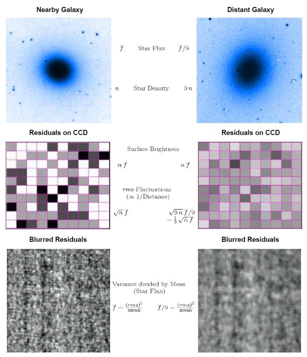 |
Figure 3. Sketch of the Surface Brightness Fluctuation method. A nearby galaxy (G1, left 1) is compared to a distant galaxy (G2, right 1) with a three times larger distance than the nearby stellar system. Note the slightly mottled structure seen in the outer parts of galaxy G1. The middle panels represent the galaxy-subtracted SBF residual view as seen on a CCD chip. One square in the image corresponds to a single CCD pixel. The bottom panels show the galaxy-subtracted SBF residuals convolved with the observed seeing to simulate the blurring caused by the earth's atmosphere. See text for a detailed description. |
From a theoretical point of view, the SBF method relies on using the ratio of the second moment to the first moment of the stellar luminosity function (LF) of the galaxy as:
 |
(2) |
with ni being the number of stars of spectral type
i and luminosity Li. The mean fluctuation
luminosity depends on
the stellar population and the galaxy colour itself depends on the
underlying population. It is important to mention that the relation in
equation 2 is very insensitive to the uncertain faint end of the
LF. Assuming asimple power-law luminosity function, the fluctuation
luminosity
scales linearly with the maximum luminosity of the stars
Li.
The primary utility of SBFs as an extragalactic distance indicator will be evaluated in Section 4. Since the data collected for SBF analysis can also be used to determine the surface brightness, which provides information about the first moment of the stellar LF, the surface brightness therefore allows a measure of the stellar content solely from the integrated flux. The utility of SBFs as stellar population tools will be discussed in Section 3.4. Further, as the SBFs also depend on the second moment of the stellar LF, the SBF signal is more sensitive to the most luminous stars in a stellar system. In case of elliptical galaxies, these stars are evolved cool giant stars. The application of SBFs as a constraint on the evolution of evolved stellar populations will be presented in Section 5.
Within a single CCD exposure of a stellar system there are a number of pixel-to-pixel fluctuations and the individual sources can basically be divided into three groups: (1) intrinsic fluctuations from the target of interest itself (e.g., a galaxy), (2) fluctuations from other objects, and (3) fluctuations caused from the instrumentation.
Intrinsic fluctuations are sources that account for additional contributions to the basic galaxy fluctuation signal and are part of the galaxy or its environment (e.g., GCs, HII regions, planetary nebulae, satellite systems (dwarf galaxies), etc). Moreover, the SBFs we are interested in and want to measure are included in this group too. Other fluctuations arise from unwanted sources (primarily foreground stars or background galaxies) that are on the same exposure as the target of interest. The third group of fluctuations originates from the instrumental setup used (telescope and optics) and the detector itself (readout noise of the CCD camera, photon shot-noise) and from cosmetic artefacts (cosmic rays, traps, defect columns, noise from the counting statistics of the flatfield exposures, or residual flattening problems after the flatfield correction). Additional Poisson noise is generated from the number of detected photons in each pixel of the target itself.
Patchy (dust) obscuration results in images that are mottled or partly obscured and affects the flux of a stellar system by creating additional variance. Smooth (dust) obscuration can reduce the derived flux and the variance we seek to measure. By restricting the SBF analysis to elliptical and S0 galaxies, the problems of patchy dust obscuration are largely reduced. Moreover, these early-type galaxies exhibit such high velocity dispersions that only dense (c)lumps endure in the fluctuation flux measurements, hence limiting possible pixel-to-pixel correlations from gravitational clumping. However, using high-S / N images with sufficient resolution at blue wavelengths (U or B-band) the contamination of dust can be firmly established and hence the SBF technique can be extended to early-type spiral galaxies or bulge-dominated galaxies.
There are two main factors of the fluctuations caused by the instrumentation used: The readout noise and the device photon shot-noise. The variance of the readout noise is given by a relation between the inverse CCD gain a (in units of electrons per analog-to-digital unit (ADU)) and the CCD readout noise NR (in units of electrons) as (Tonry & Schneider 1988):
 |
(3) |
The formula of the variance of the readout noise is composed of the
contributions from the inverse CCD gain a and the average total
signal  (x,
y) at the point (x, y) on the CCD chip in ADU. For
the mean total signal, the bias level was subtracted and the detector
response and pixel-to-pixel variations (flatfield) were corrected,
whereas the mean sky brightness has not been removed. The variance of
the photon shot-noise, which is the noise due to the photon counting
statistics, is defined as
(x,
y) at the point (x, y) on the CCD chip in ADU. For
the mean total signal, the bias level was subtracted and the detector
response and pixel-to-pixel variations (flatfield) were corrected,
whereas the mean sky brightness has not been removed. The variance of
the photon shot-noise, which is the noise due to the photon counting
statistics, is defined as
 |
(4) |
The average total signal
is denoted by the relation
=
 +
s, with
(x,
y) being the mean signal of the stellar system at the point
(x, y) in ADU and s being the sky flux.
+
s, with
(x,
y) being the mean signal of the stellar system at the point
(x, y) in ADU and s being the sky flux.
All these sources of instrumental related noise are described by a white power spectrum and can therefore be separated from the intrinsic fluctuations from the stellar component of the target system, which are represented by a power spectrum of a point-spread-function (PSF); see further Section 2.2. Intrinsic fluctuations produced from sources other than the target object (e.g., stars, globular clusters, faint background galaxies) are more difficult, because these sources are characterized by a similar power spectrum as the spatial luminosity fluctuations that we are interested in. Further, the variance signal of the luminosity fluctuations could be corrupted by the presence of spiral arms or star forming regions, which would invalidate the general assumption that adjacent pixels are independent samples of the average stellar population.
In the following, the basic procedures involved in measuring a fluctuation flux are presented. The details of the complete data reduction steps and analysis tools are beyond the scope of this review. The interested reader is therefore referred to Tonry et al. (1990, hereafter TAL90); Sodemann & Thomsen (1995); Blakeslee et al. (1999); Fritz (2000, 2002).
Distance determinations using SBFs are based on two individual steps that are linked together: (i) measurement of a fluctuation flux, and (ii) conversion to an absolute distance by assuming a calibrated, absolute fluctuation luminosity. There are several important facts regarding the SBF method:
Preferred targets are dust-free systems, like elliptical (E) and S0 galaxies, spiral bulges or globular clusters.
The total integration time must be sufficiently
long enough to collect ≥ 5 photons per source with apparent magnitude
. Moreover,
the PSF must be stable and uniform across the field during the collection
of the observations. In particular, the telescope exposure time must exceed
the point at which the photon shot noise per pixel is smaller than
the intrinsic SBFs. This breaking point is given by the time at which
1 photoelectron is collected per giant star of brightness
, with the integration
time defined as
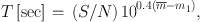 |
(5) |
where S / N represents the required signal-to-noise ratio
and m1 denotes
the magnitude for 1 detected photoelectron per second on the CCD detector.
Typically, ∼ 5-10 e− for a star with
are sufficient to
reach a S / N ∼ 5−10, and an observation
strategy with several dithered exposures is recommended to limit the
impact of possible image gradients, fringe patterns, or CCD defects. The
uncertainties in
are
defined as δ = 0.03
[(FWHM / arcsec) × d / (1000 km
s−1)]2,
with the first error term being the full-width-at-half-maximum (FWHM)
of the PSF and the second the distance d.
The photometric I-band is a useful tool for distance measurements
because the absolute fluctuation magnitude
is even
brighter than the high sky background level in the NIR wavelength
regime. The usage of this band also limits the impact of dust absorption.
Moreover, for cluster galaxies there exists an empiric relationship of
I with the
mean galaxy colour with a small scatter
(∼ 0.07 mag), which can be used to derive distances (see further
Section 3.1 and equation 9).
The calibration of the zeropoint of the absolute fluctuation magnitude
I can be
based on theoretical stellar population synthesis
models (SBF acts as a primary distance indicator) or derived from an
empirical relationship (SBF is used as a secondary distance
indicator). The empirical calibration is based on observations of
galactic GCs or LG galaxies. The methods using predictions from stellar
population prescriptions and galactic GCs are expected to be consistent
at least to the 10% level.
In practice, the basic procedure to measure a fluctuation flux is to
perform high S / N observations and data reductions in
such a way as to obtain a smooth and uniform image that is based on a
precise photometric calibration. To ensure a reliable calibration, a
significant fraction of the observing time must be devoted to
photometric standard stars. As can be seen from equation 5, the
fluctuation signal increases proportional to the exposure time and the
ideal assumption is to obtain ≥ 10 photoelectrons for a star of
in order to leave the
regime of photon-counting (shot-noise) statistics and enter the regime
of star-counting statistics. Therefore, the integration time depends
only on the SBF magnitude
and the detector sensitivity, but is independent
of the size of the target object. Hence, in the absence of a sky background
all points in a stellar system pi are described by the
same ratio of variance of fluctuations to variance of photon-counting
statistics as
p(x, y) ∝ σf2 /
σP2 + (1 + s /
).
Once the initial data reduction (including cosmic ray removal) and
photometric calibration is complete, obvious point sources, background
galaxies, any regions contaminated by CCD defects or dust are masked out
and the sky background level in the outer districts of the stellar
system is estimated using a r1/n
law profile (n = 4 for E+S0 galaxies) plus constant offset (which
allows both measurements of the mean galaxy colour and
as function of
radius). In the next step, elliptical isophotes are fitted to the masked
sky-subtracted galaxy image and a smooth galaxy model is constructed. This
galaxy model is then subtracted from the masked image and corrected for
large-scale background deviations (which affects only the low wave
numbers in the image power spectrum, which are excluded from the
determination of ) to
yield a residual image with various fluctuation contributions. From this
residual image the Fourier power spectrum is constructed and the mean
variance measured.
Before the determination of the average fluctuation variance, the contributions of fluctuations must be accounted for. Foreground stars, background galaxies, and GCs are identified and classified with an automatic photometric program to a specific completeness level (e.g., Sodemann & Thomsen 1995; Fritz 2000, 2002). Their contribution to the fluctuation amplitude of interest (P0) can be described as
 |
(6) |
with Pr being the residual fluctuation signal of
undetected point sources of faint GCs and background
galaxies. Usually the globular cluster luminosity function (GCLF) is
assumed to be Gaussian and the background galaxy luminosity function to
be a power law. Fortunately, even large uncertainties in
Pr (∼ 20%) contribute only marginally to the
final error in .
In the next step, the total fluctuation amplitude P0 is derived. The power spectrum of the masked data P(k) consists of a constant P0, multiplied by the power spectrum of the PSF E(k) and a constant P1 (from white-noise component) following the relationship (TAL90)
 |
(7) |
It is expected that there is extra noise at very low wave numbers (k ≲ 25). However, P0 is tightly constrained by the data across a wide range of wave numbers and therefore a precise measurement of the fluctuation flux and variance is possible. We also would like to emphasize that the ratio (P0 − Pr) / P1 = Pfluc / P1 represents another good indicator of the S / N level.
Finally, the fluctuation magnitude
can be derived as
 |
(8) |
Note that by using the masked residual image to create the expectation
power spectrum of the PSF, E(k), the contributions of the
target of interest, background galaxies, GCs, and dust are all excluded,
leaving the fluctuation variance σf2
dependent on the mean flux per star
f and the mean
galaxy flux per pixel N
(see equation 1).
1 ESO Online DSS2: http://archive.eso.org/dss/dss Back.