

Problem 1: Fitting a straight line to simple data
Let us assume that some theory tells us that we should expect a linear relationship to exist between some physical quantities x and y where, unfortunately, the slope and zero-point of the relationship can not be predicted by the theory - we need to use observations and statistics to estimate these missing parameters. We want to find the straight line of the form y = mx + b that "best" describes our data set, which consists of the N observed data points (x1, y1), (x2, y2), ..., (yN, yN). We can write this as
where I use the symbol "
where
then the Likelihood,
This comes straight from elementary probability theory: if
P(
Then,
This means
For the purposes of this discussion, it is convenient to write this
pair of simultaneous equations as a matrix equation. Since
so
And since
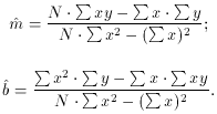
the algebraic solution to this set of equations is:
The quantity given by
is called the mean error of unit weight, and is a very useful measure
of the scatter of your data. It is essentially the root-mean-square
value of your observational errors,
If you had trouble following my derivation of the least-squares fit of
a straight line, let's look at a couple of even simpler examples, to
show how the general principle of minimizing the sum of the squares of
the residuals can be used in real life. For the first example, let us
assume that we have a set of observed values yi which
are supposed to
equal some constant. Of course, because of observational errors the
various yi will not have a single, constant value, but
instead will
show some amount of scatter. Let's derive the least-squares estimator
of that constant which "best" fits the observed yi. In
the same
notation as above, we want to solve a least-squares problem of the form
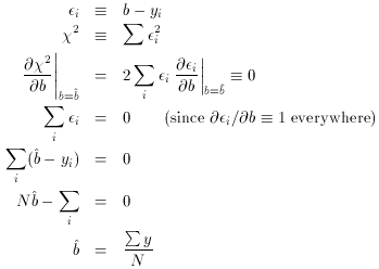
where b is the desired constant. Here are the steps:
In other words, the least-squares estimator of that constant parameter
b which best fits some set of data yi is simply
the arithmetic mean of
those yi. This is why we have all grown up always
taking the mean of a
bunch of independent measurements: it can be shown mathematically to
be the "best" way of extracting an estimate of some constant from
error-prone data, provided that the observational errors follow a
Gaussian distribution.
Now let's look at a slightly different problem. Suppose you know that
your measured quantities yi should be linearly related
to other
quantities xi (which are known to infinite precision),
but you also
know that the best-fitting line must pass through the origin: y = 0
when x = 0. One astronomical example of this kind of problem is the
calibration of the Hubble law for the expansion of the Universe: for
some set of distant galaxies we measure the radial velocities of
recession and estimate their distances, and then fit a straight line
giving distance as a function of radial velocity (for the purposes of
the present discussion, I assume that the radial velocities may be
regarded as of infinite precision in comparison with the
distances). Since our model assumes that the recession velocity must
be zero at zero distance, we have to solve a problem of the form
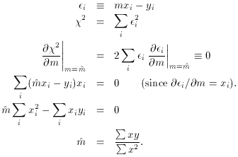
Let's do it.
This is the least-squares formula for determining the slope of a line
which is forced to pass through the origin. It is just as fundamental
as using the arithmetic mean to obtain the best estimate of a
constant, but is less familiar to most of us.

 " to
represent the phrase "is fitted to." For
the time being, we must assume that only the observable quantities
yi
contain observational errors; we must be certain that the quantities
xi are known perfectly, or at least that the errors in
the x's are
negligible in comparison to the errors in the y's. If the
observational errors in the quantities yi, which I
will denote by
  i,
follow the normal error distribution,


 1),
1),

 , of
obtaining these fitting residuals is

 i) is
the probability that the observed quantity y1 is wrong
by an amount
 i, and
P(
 2) is
the probability that observed quantity y2 is wrong by
amount
  2, and if
the error that you made in y1 is independent of the
error that you made in y2, then the probability of
making errors
  1
and
1
and  2
simultaneously is
P(
 1)
.
P(
 2). This principle may be
generalized to give the probability of observing the full set of
observational errors
 1,
1,
 2,...,
 N, which results
in the equation for
 that I just gave. The
"method of maximum likelihood" seeks the
values
  and
and
 for which
 is maximized, since
these are the most
likely values of m and b, given the current set of data. (I use the
"^" symbol to denote the specific estimate of a parameter which has
been derived from the data by some statistical method; without the
"^", the parameter is considered to be a variable). Clearly,
 is
maximized when
  i=1N,
i=1N,
 i2 is
minimized: hence, for an assumed Gaussian
error distribution, the method of maximum likelihood becomes the
so-called "method of least squares." For this sum, we often use the
symbolic representation


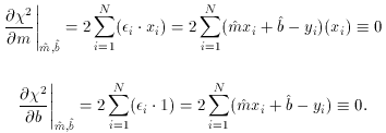
 2 is at a minimum and
the Likelihood is at a maximum when:
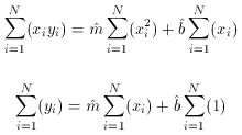
 i=1N(1) = N
we have



 i. (The
-
 i are
sometimes also
referred to as the residuals of your yi values,
but note that these
are usually considered to have the opposite sign: residual =
observation - model = yi - (mxi
+ b). Of course, when you square them,
the sign makes no difference.) The sum of the squares of these
residuals is divided by N - 2 instead of N to eliminate a
bias in the
estimate of the scatter: any two points define a straight line
perfectly, so if there are two data points the residuals from the
"best" fit will always be zero regardless of the true errors in the
yi. It works similarly for other values of N:
since we have used our
data points to determine two previously unknown quantities, the
observed scatter of the data about the best fit will always be a
little bit less than the actual scatter about the true
relationship. Dividing by N - 2 instead of N completely
removes this
bias; you can find a mathematical proof of this statement in a text on
the theory of statistics.

