A. Errors in several coordinates

The first big problem that you often run into with real data is the fact that the formulae I have presented will not work correctly unless the observational errors occur only in a single variable, which must be taken as the dependent variable, or the "y"-direction in most of the equations that I have written so far. It's true that this condition is often met, at least approximately, and we have seen some cases like this. For instance, in the radioactive-decay experiment of my first lecture we might guess that the times of the observations are accurately known, maybe through some computer-controlled clocking arrangement on the Geiger counter. In the least-squares fits of model profiles to star images which we did in the second lecture, we may assume that the x, y positions of the individual pixels are known with high accuracy, so that the scatter observed in the stellar profile is dominated by errors in the actual intensity measurements as opposed to errors caused by our ignorance of the pixel locations.

However, in many other cases both coordinates may contain significant errors. Look again at Mike Pierce's galaxy data: the three sets of points that I fit a bundle of parallel lines to in my first lecture. I really shouldn't have done that, because I violated my own conditions laid out at the beginning of the lecture: both coordinates in that diagram are observed quantities that are prone to error; it's not safe to assume that either is known well enough to put it on the right side of the equals sign. But does it matter, really? Yes, it does.

To demonstrate this let's do the solution both ways, first putting luminosity to the left of the equals sign and then putting velocity to the left, and see if we get the same straight line both times. Wanting to use appropriate weights, I asked Mike what he thought reasonable standard errors for his data were, and he told me:

"[log(L / L)] 0.04,       [log(2V)] 0.03"

(An eloquent man.) Now let's do the solution both ways, considering only the standard error of the independent variable in each case. Here are the actual results obtained from four-parameter fits, as discussed in lecture 1:

Attempt Number 1
log(L / L = m[log(2V) - 2.5] + b(type)	log(2V) = w[log(L / L) - 10] +p(type)
[log(L / L)] = 0.04	(2V) = 0.03
m = 2.9113 ± 0.1549	w = 0.27251 ± 0.01450
b(S + I) = 9.98	p(S + I) = 2.49
b(E) = 10.29	p(E) = 2.44
b(S0) = 10.37	p(S0) = 2.39
m.e.1 = 6.22	m.e.1 = 2.54

Please notice that, for the purposes of this example only, the symbol "w" does not stand for observational weight, it stands for the inverse of the slope m. I'm sorry if this change of notation causes any confusion, but I couldn't resist. I have subtracted a constant value from the independent variable in each of these two solutions (I subtracted 2.5 from log(2V) on the left, 10 from log(L / L) on the right) just so that the zero-point of each straight line would occur somewhere in the middle of the data -that is b(type) and p(type) would represent some "typical" galaxy, not some impossible galaxy with an internal velocity of 1 km s^-1 or a luminosity of 1 L. However, in the following discussion, I plan to de-emphasize the zero-points of these relations as astrophysically "uninteresting," and worry about only the slopes, at least for the time being.

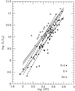
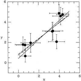
If the method of least squares is a magic machine for finding the one "best" straight line corresponding to a given set of data, then we must have w^-1 = m, right? Well, is that what we get? If you whip out your pocket calculator and punch the numbers in, you'll find that (0.27251)^-1 = 3.6696 not 2.9113. Both these families of straight lines are illustrated in Fig. 3-1, where the left-hand solutions (luminosity as a function of velocity) are shown as solid lines, and the right-hand solutions (velocity as a function of luminosity) are shown as dashed lines. You can even use some of that propagation of errors stuff to show that (w^-1) = (w) / w² = 0.1953. So not only are the two slopes significantly different, they are different at something like the 4.5 level, even though both solutions are based on exactly the same data! Still believe that least squares is the magic solution to all your data-reduction problems?

Figure 3-1.

You might also have noticed that the m.e.1's of these two solutions are pretty far from unity. Maybe that's because in each case we have considered only part of the observational errors: in the case of log(L / L) = m[log(2V) - 2.5] + b, for instance, a given data point will lie off the mean straight line not only because of errors in log(L / ), but also because of errors in log(2V). If we really want to do the solution right, we must include both these standard errors in evaluating the fit. From propagation of errors we can easily demonstrate that if

then

m - before we can do the solution. But you can guess how we'll handle that: successive approximation! We take a wild guess at the slope (the value we got from Attempt Number 1, maybe?), compute new weights for all the points, redo the solution, use the new m to reweight all the points, and do it again and again until the answer stops changing. Surely that will solve all our problems! So here we go:

Attempt Number 2
log(L / L = m[log(2V) - 2.5] + b(type)	log(2V) = w[log(L / L) - 10] + p(type)
2 [] = w2(0.04)2 + (0.03)2	[] = w2(0.04)2 + (0.03)2
m = 2.9113 ± 0.1549	w = 0.27251 ± 0.01450
B(S + I) = 9.98	p(S + I) = 2.49
b(E) = 10.29	p(E) = 2.44
B(S0) = 10.37	p(S0) = 2.39
m.e.1 = 2.59	m.e.1 = 2.38

The mean errors have changed, but the answers haven't! What has gone wrong? Well, think about it. In changing the standard errors of the points in the luminosity fit from 0.04 to sqrt[m²(0.03)² + (0.04)²], we have changed the weight of each point from 1/(0.04)² to 1/[m² (0.03)² +(0.04)²]. The weights may have changed, but the weight of every point is still the same as the weight of every other point, regardless of what m is. This is the equivalent of simply adopting a different scaling parameter s in the definition of those weights. As we saw before, changing s doesn't affect the least-squares solution at all, because it can be pulled out of the summations and it always cancels out. So we get the same answer, and have exactly the same problem of unequal straight lines as we had before.

We must try to figure out why this problem occurs before we can work out a solution to it. Let's back up a step and take another look at our original equations of condition:

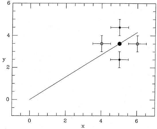
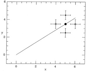
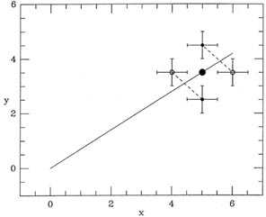
(Note that w_i has now gone back to its original meaning of weight.) At the same time, take a look at Fig. 3-2 and consider some data point lying toward one end of the distribution. The large dot lying on the line represents the "true" position of that data point, as it would be seen if it could be observed with absolutely no errors. Now, a random observational error in the y-coordinate can move the observed position of this point either up or down (closed dots with error bars); the probability of these two observational errors will be equal, provided that the error distribution is symmetric. (Please note that for this argument to be valid, there is no need to assume that the error distribution is Gaussian, merely that it is symmetric.) One of these observing errors will contribute a positive _i to the two summations above, and the other will contribute a negative _i. As I said, the probability of each of these two observations is equal as long as the error distribution is symmetric; given enough independent observations, these random errors will tend to cancel, and in the long run least squares will give the right answer on average, provided that the observational errors occur only in the vertical direction.

However, if errors can also occur in the horizontal direction, the observed position of the point could also be shifted to the left or right of its true position (open circles with error bars), as well as above or below the true position. Again, one of these points will contribute a positive _i to the summations and the other will contribute a negative _i, and again the probabilities will be equal for equal |_i|, provided the error distribution is symmetric. However, in this case the errors do not cancel. In the first of the two condition equations above, because the e_i, are multiplied by the observed x's of the points, one of the two 's - the one belonging to the point which has been scattered to the right - will make a larger contribution to the first summation than the belonging to the point which has been scattered to the left. The point at the right will exercise more leverage on the line than the point at the left, and will tend to pull the end of the line down, making its slope too shallow. If you turn Fig. 3-2 over, and consider the case of a point whose true position is near the left end of the relationship, you'll find a mirror-image situation which leads to the same result: the vertical errors cancel, but that observation whose horizontal error has scattered it away from the centroid of the observed data points will exert more leverage on the slope than the one whose error has scattered it toward the centroid of the data. Again, this excess leverage will tend to make the slope too shallow. This is the general rule: When observational errors occur in the horizontal direction, there is a strong, systematic tendency to underestimate the slope of the mean relationship. This is because we use the observed x coordinate of the point to evaluate the summations. We do this because it is what all the recipes in the standard cookbooks on "Statistics for Scientists" tell us to do (and this is what the referee of our paper expects us to do), and we forgot to remember that this only works if the errors are confined strictly to the vertical dimension.

Figure 3-2.

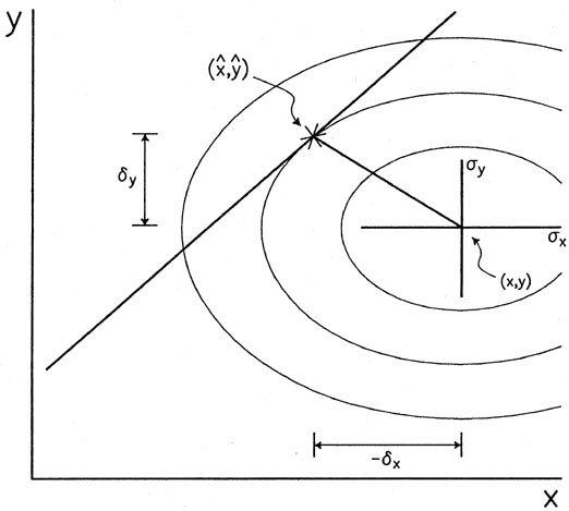
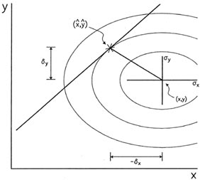
But we don't know what the _i are, all we know is the x_i. So how on Earth can we solve our problem? Well, again I'm afraid that we'll have to iterate a little. We must start off with some crude estimate of the best-fitting straight line - maybe the one obtained by pretending that ordinary least squares is OK. Then we go through the rigmarole illustrated in Fig. 3-3. Imagine that our data point sits under a bell-shaped surface representing the probability of all possible combinations of errors, _x and _y; the equal-probability contours of that surface are ellipses, three of which are shown ⁽³⁾. The straight line in the figure represents our current estimate of the linear relationship between the "true" values of x and y. The most likely position of the "true" value of this data point on the current assumed relationship is that point where the straight line penetrates most deeply into the nest of error ellipses surrounding the point's observed position: it is the place - marked with a star - where the current estimate of the best straight line touches the innermost error ellipse that it ever gets to.

Figure 3-3.

As an alternative - mathematically more correct - visualization, you might like to take a more literal interpretation of the Principle of Maximum Likelihood: the best estimate of the "true" position of the data point is that position on the line such that, when that "true" position is assumed to be correct, the probability of the observed position is maximized. To illustrate this version of the statement, imagine taking the nest of error ellipses away from the data point. Now imagine sliding the whole set of error ellipses up and down along the current guess at the best straight line, keeping the center of all the ellipses strictly on the line itself. Where does the center of all these error ellipses lie, when the smallest possible ellipse is touching the data point? I think you can convince yourself that it is exactly the same starred point (, ) that I've indicated in Fig. 3-3.

Now let's figure out where this starred point is, shall we? If you have a data point with observed coordinates (x, y) and standard errors _x and _y and if you have a provisional best-fitting line with slope m₀ and y-intercept b₀, then we have the situation which I've shown in Fig. 3-3. The equation for the line is

and the equation for any of the ellipses is

where _x = - x and _y = - y - the difference between the point's observed coordinates and its most likely "true" coordinates. (This assumes that the errors in x and y are independent. It is perfectly straightforward to develop an analogous solution for correlated errors, but the extra algebra is a little more than I want to go into right now.) Of course, the particular error ellipse that we want is the one with the smallest possible value of "constant"; this ellipse will be tangent to the straight line, since if the line crosses over the ellipse, it will obviously get the chance to touch still smaller ellipses. One condition for the ellipse to be tangent to the straight line = m₀ + b₀ is

The derivative of the ellipse equation is

so the slope at any point on the ellipse is

which gives us

The other condition for the ellipse to be tangent to the line is

which I'll use in a minute.

Now, we have to take a moment and rethink what we mean by our analytic "model," and by the observed data point's residual. If we can really have errors in more than one of our observational variables, then all the magic has gone out of the left side of the equals sign. If we can put error-prone quantities on the right, then we can put error-free quantities on the left! We can even put zero on the left of the equals sign if we want to, and what physical constant is known better than zero? By which I mean to say: if we want to, we can right our fitting equation in the form

What could be fairer than this? The observations x and y - two error-prone quantities if ever I saw any - are both together on the same side of the equals sign, with neither one receiving any sort of preferred status. Now, if our data point should really lie at (, ), and has been observed at (x, y) = ( - x, - y), what is the distance of the point from the provisional curve? Well, if our current analytic model is

and our observation is

then to first order the net observational error of the point is given by

Now you think I'm completely out of my mind. Anyone can see that the residual of the point is the same as it's always been,

right? Wrong! What matters is not how far the observed data point is from the model curve in the vertical direction, it is how far the observed point is from the "true" point - that's what tells you what the observational errors are, which in turn tell you the probability of getting that observation. The distinction becomes more obvious when we fit more complex curves than straight lines. Suppose, for instance, we were fitting a parabola to these data. The parabola might curve up sharply between and x, making it appear to be a BIG residual, when in fact the point had only been shifted a little to the side. It's not how far your data point is below the curve that matters, it's how far it is from where it belongs. So henceforth we will need to recognize the distinction between the true residual, , and the apparent residual, y.

Now, it just so happens that in this particularly simple case, where we are fitting a straight line to the data, the true and apparent residuals are equivalent:

However, as I said, this will not be true for any function other than a straight line. If I now write the second equation for tangency as

you can easily see that

We're almost home now.

Here it comes . . .

At last we can compute from known, assumed, or observable quantities - the 's and y -the most likely "true" position that the data point would have had on our assumed straight line, if only the point had no observational errors. We can now compute = x + _x (and = y + _y, though we don't need it). And finally, with our newly improved guess at where the point should be, as distinguished from where it is, we can use our good ol' least-squares techniques to compute corrections to the parameters of the line:

(Oh! those darned minus signs.) Iterate! Use the provisional line to improve our information of where the point ought to be! Use the improved x coordinates of the points to improve the estimate of the line!

Figure 3-4.

Fig. 3-4 shows how Fig. 3-2 looks at the end of this mess, with short dashed line segments illustrating the data points' final residuals. As long as all "observed" data points on a given error ellipse around the true point are equally probable - and this is true by definition - then in the long run, with enough data, the errors will tend to cancel out: there is no net torque remaining on the model to twist it away from the right answer. The only thing that you have to remember in order to create this happy circumstance is that the real, genuine maximum-likelihood condition equations are

It doesn't much matter how you approach the ultimate parameter values. Once these conditions have been met, you have the "best" parameters for your straight line.

Let me show you some simulations that I ran to demonstrate this methodology. I made up a bunch of synthetic data satisfying the condition

Just for simplicity in understanding what is going on, and with no loss of generality, I arbitrarily set m 1 and b 0. I then generated random observational "errors" in x and y,

where the size of the standard errors were themselves chosen at random:

just to illustrate that this works for unequal standard errors. I generated 5,000 sets of 10 data points having these properties, and fit straight lines to them using standard least-squares and considering only the standard errors in the y-coordinates; then I fitted straight lines again using standard least squares, but this time considering the errors in both coordinates, and iterating to get the slopes and relative x- and y-error contributions right; last, I fitted them using the scheme I outlined above, where the equations are based not on the points' observed x coordinates, but rather on their projected most-likely "true" coordinates . Fig. 3-5 shows the data points and derived solutions for one typical sample of ten synthetic observations; the steepest slope, represented by the solid line, is found with the true maximum-likelihood technique I have just described.

Figure 3-5.

Figure 3-6.

Figure 3-7.

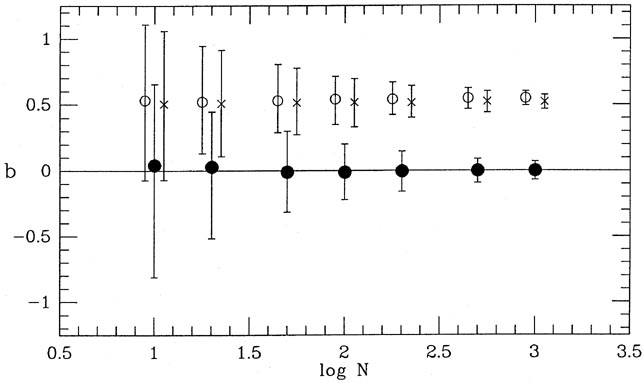
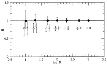
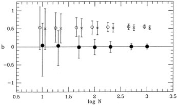
I repeated this experiment, generating 5,000 samples apiece for sample sizes of 20, 50, 100, 200, 500, and 1,000 data points. The results of this test are shown in Figs. 3-6 and 3-7, where the range of recovered slopes and zero-points are shown as functions of sample size. In each case, the open circle shows the median recovered parameter value for the first type of solution, considering only the errors in y - ²() = ²(y); the x's show the median parameter values for the second type of solution - ²() = ²(y) + m²²(x); and the closed circles show the median recovered parameter values for the least-squares solutions based upon the maximum-likelihood "true" x-values for the points. In each case, the error bars represent ±32% ( ±) ranges for the recovered parameter values. As you can see, both of the first two types of least-squares solution systematically underestimate the true slope of the relation, just as I described above. Furthermore, this bias does not go away for larger and larger sample sizes. No matter how many data points you have, the bias remains the same: the slope is underestimated by about 20%, under the present hypothesized conditions < (x) > 0.75, x_max,true - x_min,true < 5. The bias is just about equal to the standard error of the slope for a single solution based upon ten data points, but the systematic error dominates over the random errors for larger sample sizes. You may reasonably imagine that the bias would be even greater for larger values of

and smaller for smaller values of this ratio. The true maximum-likelihood technique has no such bias.

Because in this example the data points are concentrated to the right of the y-axis, when the cookbook least-squares algorithms underestimate the slope, they also cause the fitted line to intersect the y-axis too high (cf. Fig. 3-5). Again, this bias does not occur for the true maximum-likelihood technique.

So what does this method give us when presented with Mike Pierce's galaxy data?

Attempt Number 3
log(L / L) = m[log(2V) - 2.5] + b(type)	log(2V) = w[log(L / L) - 10] + p(type)
2[] = (0.04)2 + m2(0.03)2	2[] = (0.03)2 + w2(0.04)2
[log(2V)] = {-m2[log(2V)]} / {m2 2[log(2V)] + 2[log(L / L)]}	[log(L / L)] = {-w2[log(L / L)]} / {w22[log(L / L)] + 2[log(2V)]}
m = 3.5585 ± 0.1843	w = 0.28102 ± 0.01455
b(S + I) = 10.01	p(S + I) = 2.50
b(E) = 10.21	p(E) = 2.44
b(S0) = 10.41	p(S0) = 2.39
m.e.1 = 2.38	m.e.1 = 2.38

Whip out your pocket calculators and compute w^-1 and (w) / w² and tell me if you don't think we've done the right thing. Yes, we did!

There is still a problem, however. Did you spot it? The problem isn't with the analysis, it's with the data. Do the best we can with the least squares, Mike's data still come up with m.e.1 = 2.38 - the scatter is more than twice as large as it should be. So Mike has either underestimated the errors of some of his data, or there is some cosmic scatter in the relationship between luminosity and internal velocity. If the errors are underestimated, which ones are wrong? If you believe the velocities are fine and the luminosities are poor, you'll get one value for the true slope, but if you assume the luminosities are fine and the velocities are scrod up, you'll get another value for the slope. It's not simply that what you believe about the random errors of your data can affect your confidence in the answer, but rather your knowledge of the errors can affect the answer itself! Good values for the standard errors are nearly as important as good values for the observations.

Suppose that Mike has correctly estimated his standard errors, and that the problem is a cosmic dispersion in the luminosity-velocity relationship? Well, then, which do you prefer to believe? That there is a range of internal velocities among galaxies of the same luminosity? Or that there is a range of luminosities among galaxies of the same internal velocity? The way in which you answer these questions will affect the maximum-likelihood slope that you derive from the data.

Before I leave the subject, I must stress once again: the correct formulae for relating an observed datum to its maximum-likelihood true values are

where, to first-order approximation

(This can easily be - and has been - generalized to problems where any number of observable quantities - not just two - can include observational errors: Jefferys 1980.) As you can see, in fitting any function other than a straight line, we are caught in the same old bind: we can't get the "true" coordinates of the point until we have the residuals, and we can't get the residuals until we have the true coordinates. For a straight line - and for a straight line only - we can use = y (since we can observe y, given a first guess at the model), which results in the machinery I have just described. For any other function we must - can you guess? - Iterate! We postulate a model curve of the form,

guesstimate by evaluating ðF / ðx and ðF / ðy at the location of the observed datum, (x₀, y₀) (I'll have to change notation for the moment and call the observed data point (x₀, y₀). You'll see why right away.) From this we can compute provisional residuals x and y -> a new, improved datum, (x₁, y₁). Now this revised point will not, in general, be on the model curve, but it should be closer than (x₀, y₀) was. We evaluate ðF / ðx and ðF / ðy at this point, compute a new x and y, and ... We keep iterating until we finally arrive at a point (, ) which does satisfy our current model, F(, ; m₀, b₀) 0. Then we are ready to perform one more iteration of the least-squares solution, for the refinement of the model itself.

This is not "fudging" your data! The correct statement of the maximum likelihood condition is, "If my model is the best that money can buy, and if I assume that each data point should lie on the model, then the probability of finding them where they appear to be is maximized." It's simply a matter of twitching the model, and then staggering from where the points appear to be to where they most probably ought to be, so we can compute the likelihood of the observations. The residuals are always computed from where they appear to be to where they ought to be, and it is only our estimate of where they "ought" to be that we are adjusting so as to maximize the likelihood.

Since this method employs the Taylor approximation

it is not exact! However, it is still better than anything else on the market, and it is good enough for government work as long as the curvature of the model is small within the area spanned by the scatter of the data:

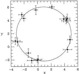
and so on. I have even used this method to fit circles to data with errors in both coordinates:

where x₀, y₀, and R were free fitting parameters (Fig. 3-8). Now, you can imagine that as the error bars become big compared to the radius of the circle, random observational errors will cause the observed data to fail outside the circle slightly more often than they fall inside the circle, so that a first-order least-squares fit to the data will tend to overestimate the circle's radius by a tiny amount. A second-order expansion would give an exact fit, but first order is good enough provided the errors are small compared to the circle (as illustrated).

Figure 3-8.

This is the place to point out another subtlety and to confess to another sin. Whenever your estimate of the error of some observable quantity depends upon the value of that quantity, the error must be evaluated on the basis of the estimated maximum-likelihood "true" value, not on the basis of the observed value. Do you remember back in Lecture 1, in the radioactivity example, where I observed N_i counts in some interval and said that this result was uncertain by ±N_i? This was wrong and I shouldn't have done it. Why? Well, suppose that the true expected number of radioactive decays in some interval was 100 counts. In identical repeated experiments you'll sometimes get more than 100 counts, sometimes less, just because of Poisson statistics. With essentially equal probability, you could get 90 counts in that interval, or you could get 110. If you then weight these observations according to the observations themselves, you'd say the first observation was 90 ±90, and the second was 110 ±110 - the first observation would get more weight than the second in spite of the fact that in Truth they are equally likely. In fitting a large ensemble of data, you wind up systematically underestimating the truth. For maximum likelihood to work, you must assume the truth of the model in evaluating the likelihood of the observations, and it is this likelihood which must be maximized. Iterate! Sure, you can start out by weighting the data according to their observed values, thus:

but then derive your error estimates from the current model, not from the data:

(Of course, if you are doing anything more complicated than a straight mean - such as fitting exponentials - it will take more than one iteration to get it right.) This works in general, and I can't repeat it enough: for maximum likelihood to work, you must assume the truth of the model, including its implications as they regard "true" values and the standard errors of your observed quantities. This gives the likelihood which must be maximized.

³ In stating that the equal-probability contours are ellipses, I have assumed that the error distributions in x and y are the same, to within scale-length constants which may be represented by some constants _x and _y. It is not necessary to assume that these error distributions are Gaussian in form. Back.