


A Statistician: is ``a man prepared to estimate the probability that the Sun will rise tomorrow in the light of its past performance'' (3). This definition, which I admit to taking out of context, is by an eminent statistician; it may confirm our worst suspicions about statisticians eminent or otherwise. At the very least it should emphasize care of definition - what is tomorrow when the Sun does not rise? Let us be more careful:
``Statistics'' is a term loosely used to describe both the science and the values. In fact, the science is
Statistical Inference: the determination of properties of the population from the sample,
while
Statistics are values (usually, but not necessarily, numerical) determined from some or all of the values of a sample.
Good statistics are those from which our conclusions concerning the population are stable from sample to sample, while good samples provide good statistics, and require appropriate design of experiment.
The ``goodness'' of the experiment, the sample, or the statistic is indicated by the
Level of Significance: suppose we perform an experiment to distinguish between two rival hypotheses, the null hypothesis (H0; ``failure'', no result, no detection, no correlation) and its alternative (H0; ``success'', etc.). Before the experiment we make ourselves very familiar with ``failure'' by determining, assuming H0 to be true, the set of all possible values of the statistic under test, the statistic we have chosen to use in deciding between H0 and H1. Furthermore, suppose that when we do the experiment we obtain a value of the statistic which is ``unusual'' in comparison with this set, so unusual that, say, only 1 per cent of all values computed under the H0 hypothesis are so extreme. We can then reject H0 in favour of H1 at the 1 per cent level of significance. The level of significance is thus the probability of rejecting H0 when it is, in fact, true.
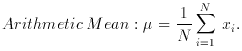
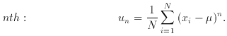
Now consider N values of xi where i = 1, 2 . . . N and x may have a continuous or a discrete distribution. The following definitions are general:
1. Location measures
Median: arrange xi according to size; renumber. Then
Mode: xmode is the value of
xi occurring most frequently.
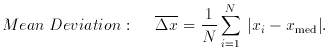
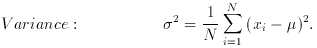
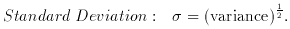
2. Dispersion measures
3. Moments
(Moments may be taken about any value of x; those about
the arithmetic
mean as above are termed central moments.) Note that
µ2 =
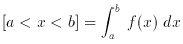
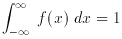
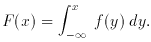
Finally, consider probability distributions: if x is a continuous
random variable, then f (x) is its probability density
function if it meets these conditions:
and
In the study of rounding errors, and as
a tool in theoretical studies of other continuous distributions.
x is the number of ``successes'' in an
experiment with two possible
outcomes, one (``success'') of probability p, and the other
(``failure'') of probability q = 1 - p. Becomes a Normal
distribution as n -> The limit for the Binomial distribution as
p << 1, setting µ The essential distribution; see text. Central
Limit Theorem ensures
that majority of ``scattered things'' are dispersed according to f
(x;µ, Vital in the comparison of samples, model
testing; characterizes the
dispersion of observed samples from the expected dispersion, because
if xi is a sample of For comparison of means, Normally-distributed
populations; if n xis
are taken from a Normal population (µ, For comparison of two variances, or of more than
two means;
if two statistics (
Probability densities and distribution functions may be similarly
defined for sets of discrete values x = x1,
x2. . . .xn, and for
multivariate distributions. The better-known (continuous) functions
appear in Table 1, together with location and
dispersion measures - note
that the previous definitions for these may be written in integral form
for continuous distributions. The table includes some indication of how
and/or where each distribution arises, and for most of them, I avoid
further discussion. But there is one whose rôle is so fundamental that
it cannot be treated in such a cavalier manner. This follows in the next
section.
xmed
= xj where
j = N / 2 + 0.5, N odd
= 1/2 (xj + xj+1 where
j = N / 2, N even.
 2; this and
the next few moments characterize a probability distribution (defined
below). The first two moments are useless, since
µ0
2; this and
the next few moments characterize a probability distribution (defined
below). The first two moments are useless, since
µ0  1
and µ 0.
1
and µ 0.
Skewness:  1 = µ32
/ µ23 indicates deviation from symmetry;
1 = µ32
/ µ23 indicates deviation from symmetry;
= 0 for symmetry about µ.
Kurtosis: 2 = µ4 /
µ22 indicates degree of peakiness;
= 3 for Normal distribution.
Distribution
Density function
Mean
Variance
Raison d'Être
Uniform
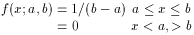
(a+b)/2
(b-a)/12
Binomial

np
npq
 .
.
Poisson

µ
µ
np. It is
the ``count-rate'' distribution, e.g. take a star from which an average
of µ photons are received per  t (out of a total of n emitted; p << 1);
the probability of receiving x photons in a t is f
(x;µ). Tends to the
Normal distribution as µ -> .
t (out of a total of n emitted; p << 1);
the probability of receiving x photons in a t is f
(x;µ). Tends to the
Normal distribution as µ -> .
Normal (Gaussian)

µ
2
).
Chi-square
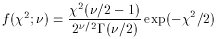

2
variables Normally and independently distributed
with means µi and variances i, then 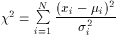 obeys f (
 2; )
Invariably tabulated and used in integral form. Tends to Normal
distribution as -> .
2; )
Invariably tabulated and used in integral form. Tends to Normal
distribution as -> .
Student t

0
/(-2)
(for > 2)
), and if xs and
s are found
as in text, then t = 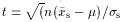 is
distributed as f (t,)
where ``degrees
of freedom'' = n -
1. Statistic t can also be formulated to compare
means for samples from Normal populations with same , different µ
(4). Tends to
Normal as -> .
is
distributed as f (t,)
where ``degrees
of freedom'' = n -
1. Statistic t can also be formulated to compare
means for samples from Normal populations with same , different µ
(4). Tends to
Normal as -> .
F
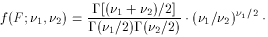
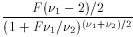 2/(2-2)
(for 2 > 2)
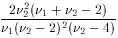 1
and 2) each follow the
Chi-square distribution,
then
1
and 2) each follow the
Chi-square distribution,
then  is distributed as
f(F;1,2). Care required in application;
see (4),
(9).
is distributed as
f(F;1,2). Care required in application;
see (4),
(9).