4. DETECTION OF SIGNAL

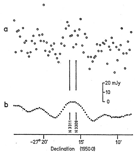
Fig. 3 (a) shows data obtained by ``stacking'' 50 continuum scans in declination with the Parkes 64-m telescope operating at 5 GHz. It represents an attempt to detect emission from the pair of galaxies NGC 3309 / 3311, whose declinations are as marked, One aspect of the observation is indisputable - noise is present. But is signal? The search for molecular lines at particular frequencies is an analogous problem; the output of the many channels of a digital correlator is a record which may look similar to Fig. 3 (a), but in the frequency domain instead of the spatial. Is interstellar rhubarb present at the predicted frequency? Digital spectrophotometry provides similar records and detection problems in optical astronomy.

``Success'' in such experiments is usually described as a detection at the ``2'' level, the ``3'' level, etc. This is, of course, a direct reference to the Normal distribution; success at the 2 level means that there is signal present at an amplitude of twice the standard deviation of the ``noise''. But why can we invoke the Normal distribution to describe the ups and downs of the record? It is because we can reasonably expect these fluctuations to be ~ Normally distributed. In radio astronomy, the Central Limit Theorem does the trick: the weak signals collected by the radio telescope have dominating fluctuations imposed upon them by noise voltages in the first stages of the receiver. But each data point emerging from the receiver is the result of some averaging via our ``output time-constant'' (low-pass filter), which thus produces (for stable atmospheres and receivers!) a set of fluctuations close to Normal in distribution. (In the observations of Fig. 3 (a), the unsmoothed receiver output was rapidly sampled at 10 ms intervals, and each point shown is the average of many such samples.) In optical astronomy, the limit of the Poisson distribution does the trick: optical astronomers are notoriously short of photons, but those which they receive are strong, so that the output fluctuations reflect not receiver characteristics so much as the Poisson statistics of the ``events'' of photons arriving. As soon as there has been enough integration to collect more than an average of 10 events per sample interval, we are talking about fluctuations distributed ~ Normally. (This may be viewed as a particular instance of the operation of the Central Limit Theorem, differing from the radio astronomer's case only in that the underlying probability distribution is known.)

Fig. 3(a) The sum of 50 scans in declination, 2°.5 min-1, to detect the galaxy pair NGC 3309 / 3311 with the Parkes 64-m telescope at 5 GHz. (b) The observations after application of a digital filter to attenuate spatial frequencies above those present in the telescope beam. The vertical lines indicate the declinations of the optical images.

In this regard, then, consider the astronomer's most common level of ``success'' - the infamous ``2 result''. Table III gives the area left under the Normal curve in the tails beyond various multiples of , and it tells us that 4.6 per cent of the area lies outside the ± 2 limits. A ``2 result'' therefore occurs by chance 4.6 times out of 100. In most cases we know the sign of the result (if there is a result) - the molecular or atomic transitions are predicted to be seen either in emission or absorption; radio emitters yield positive flux densities. Thus the chance probability becomes the area under only one of the two tails, and drops to 2.3 chances in 100 of arising by chance, or about one in 50. The genuine 2 result is thus believable, and usually one or two other factors can be adduced. Is the deflection the appropriate breadth, namely that of the predicted line-width, or of the telescope

Table III
The tails of the Normal distribution

	Percentage area under the Normal curve in region:
m	> m	> m, < -m	-m < x < m
	(one tail)	(both tails)	(between tails)
0	50.0	100.00	0.0
0.5	30.85	61.71	38.29
1.0	15.87	31.73	68.27
1.5	6.681	13.36	86.64
2.0	2.275	4.550	95.45
2.25	0.621	1.24	98.76
3.0	0.135	0.270	99.73
3.5	0.0233	0.0465	99.954
4.0	0.00317	0.00633	99.9937
4.5	0.000340	0.000680	99.99932
5.0	0.0000287	0.0000573	99.999943

But we do not; and, indeed, astronomers feel it necessary to quote 3 and up to 7 results, for which the probabilities of chance occurrence (Table III) are ludicrously small (e.g. 1.3 chances in 1000 for the chance 3 result, one-tail test). The problem arises because: (a) all observers are biased (otherwise we would never bother to observe at all), and (b) none can estimate noise properly. Accusation (a) at its most libellous is - how many times did the astronomer make the observation before he got the particular result reported? Alternatively, did he make just one observation, terminating the integration when the ``expected'' result was obtained? (Note that this latter point constitutes a reasonable argument against the use of on-line data displays.) Both, of course, lead to overestimation of significance. Accusation (b) can be considered with more sympathy. In the course of any observation, something (e.g. interference, clouds) is bound to upset the underlying probability distribution for a proportion of the time, albeit small, and, in so doing, destroys the ability of the Central Limit Theorem to guarantee a Normal distribution. It may be obvious which portion of the record has been affected, and the offending points (presumably well displaced from the critical region of the record) can be rejected from the calculation of . But it may be less obvious. For instance, in Fig. 3 (a), the highest point is so far removed from its neighbour that it is clearly the result of a short-term change in the underlying distribution, and few would argue against its exclusion from a estimate. But what about other points? Rejecting one or two or several points a posteriori and with no physical justification starts you on the Slippery Slope; equally evil is choosing a ``nice quiet bit'' of the record for the noise estimate. It is advisable to adopt an a priori procedure, to state exactly what this is, to present as much of the data as practicable (one picture is worth 1000 numbers) and, in the light of (unhappy) experience, to be pessimistic rather than optimistic. So much for your own results; for the interpretation of those of others, there is a strong case for knowing the observer.

Rigorous hypothesis testing, then, as described in most books on statistics (e.g. (1), (4)) is not easy to apply to the question of signal detection. However, the essence of signal detection lies elsewhere, and there is a considerable literature, e.g. (6), (7). The secret to success consists of knowing the answer, and then filtering away extraneous information to improve the signal/noise ratio of this answer. The ``answer'' consists of the Fourier components in the data array which the sky + telescope can produce; and, indeed, some of these possible components can be rejected specifically if the observer is not interested in them (or accidentally if he is not aware that they could exist in the first place). The filtering process reduces the amplitude of the unwanted Fourier components; it always results in some loss of information, because ``unwanted'' and ``wanted'' components must overlap somewhere in the frequency domain. The filtering may be done mechanically, electronically or digitally. Nowadays it is common to let the recording gear obtain the data with minimal treatment, and to deal with it digitally later.

Consider for example the record of Fig. 3 (a). It contains noise (plenty!), some baseline drift, and perhaps some signal (not enough!). Therefore we want to suppress the highest spatial frequencies, which are clearly noise and are much higher than those contained in the Fourier Transform of the telescope beam (FWHP 4 arcmin), and the lowest spatial frequencies, those of wavelength comparable to the record length. Let us deal first with the noise. For this we need a low-pass digital filter; such a thing consists simply of a set of ``weights'', and each ``filtered'' point is obtained as the weighted mean of itself and an equal small number of its neighbours on either side - here five points either way were used; if xf_i are the filtered points and x_i the original points,

The weights w_j (< 1, calculated as described by Martin (8) were designed to give a relatively severe filter with no overshoot and with a half-power width about one-half that of the telescope beam, producing some consequent loss of resolution. The effectiveness in dealing with the noise is shown by Fig. 3(b). (A simpler filter which avoids the question of design almost entirely is surprisingly effective: simply average each point with its neighbours, and avoid severe loss of resolution by choosing a small number of neighbours (symmetrically!) so that the width of this ``square'' filter (all w_j = 1) is less than, say, one-half of the width of expected features.)

Now for the high-pass filter to fix up the baseline - or is it necessary? For short records such as this, a linear adjustment of the baseline is probably satisfactory: average several points at each end; fit a straight line; and subtract it from all points. Clearly this changes Fig. 3 (b) in the same way as a slight tilt of the page, and adds little to the interpretation - an approximately beamshaped deflection at about the right position indicates detection of NGC 3309 / 3311, confirmed independently at 5 GHz using an entirely different observational technique. High-pass filtering to remove the very low frequencies may be important for longer records whose lengths exceed the scale of individual features by large factors. The process usually consists of baseline or continuum estimation and subsequent subtraction. A commonly advocated method is to carry out least-squares fitting of a polynomial (e.g. (9)). In practice this may prove to be messy, and heavy smoothing provides a better way. This consists of constructing a ``baseline array'' in which each point is the average of the corresponding point in the data array and many of its neighbours on either side, say out to ±3 or 4 times the expected scale of the features. (Accuracy may be improved by using weighted heavy smoothing, and by ``patching'' over regions where there are obvious features.) Fig. 4 demonstrates the effectiveness of this technique in high-pass filtering of long continuum-scans in radio astronomy. It works for any continuum for which features occupy < 50 per cent and, in particular, provides a good way of estimating optical continua for digitized spectra.

Fig. 4. Steps in the on-line processing (10) of a scan recorded in the course of the Parkes 2.7-GHz survey for extragalactic sources. In the survey a twin-beam system was used in which the receiver recorded the difference between signals at the two feeds of the 64-m telescope; hence the appearance of ``positive'' and ``negative'' sources on the records. Scan A - as recorded from sampling of the receiver output; scan B - after application of a low-pass filter to attenuate noise frequencies; scan C - after baseline removal (high-pass filtering) consisting of the construction of a baseline array by heavy smoothing, and the subtraction of this array from scan B.