


4.3. The results of coherence
Having presented the toy model, let as look at the behavior of the
real cosmological variables. Figure 8 shows

 (the photon
fluctuations) as a function of (conformal)
time
(the photon
fluctuations) as a function of (conformal)
time  measured in units of
*, the
time at last scattering.
measured in units of
*, the
time at last scattering.

|
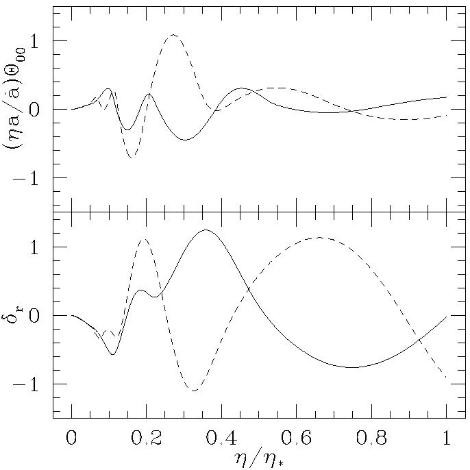
Figure 8. The evolution of |
Two different wavelengths are shown (top and bottom panels), and each panel shows several members of an ensemble of initial conditions. Each curve shows an early period of growth (squeezing) followed by oscillation. The onset of oscillation appears at different times for the two panels, as each mode ``enters'' RJ at a different time. As promised, because of the initial squeezing epoch all curves match onto the oscillatory behavior at the same phase of oscillation (up to a sign). Phases can be different for different wavelengths, as can be seen by comparing the two panels.
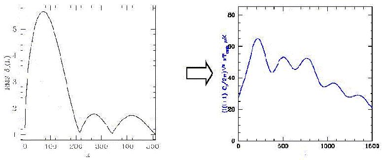
To a zeroth approximation the event of last scattering simply releases a snapshot of the photons at that moment and sends them free-streaming across nearly empty space. The left panel of Fig. 9 (solid curve) shows the mean squared photon perturbations at the time of last scattering in a standard inflationary model, vs k.
|
Figure 9. The left panel shows how temporal
phase coherence manifests itself in the power spectrum for
|
Note how some wavenumbers have been caught at the nodes of their oscillations, while others have been caught at maxima. This feature is present despite the fact that the curve represents an ensemble average because the same phase is locked in for each member of the ensemble.
The right panel of Fig. 9 shows a typical angular power
spectrum of CMB anisotropies produced in an
inflationary scenario. While the right hand plot is not exactly the
same as the left one, it is closely related. The CMB anisotropy power
is plotted vs. angular scale instead of Fourier mode, so the
x-axis is ``l'' from spherical harmonics rather than k. The
transition from k to l space, and the fact that other quantities
besides affect the
anisotropies both serve to wash out
the oscillations to some degree (there are no zeros on the right plot,
for example). Still the extent to which there are oscillations
in the CMB power is due to the coherence effects just discussed.
As our understanding of the inflationary predictions has developed, the defect models of cosmic structure formation have served as a useful contrast [12, 13]. In cosmic defect models there is an added matter component (the defects) that behaves in a highly nonlinear way, starting typically all the way back at the GUT epoch. This effectively adds a ``random driving term'' to the equations that is constantly driving the other perturbations. These models are called ``active'' models, in contrast to the passive models where all matter evolves in a linear way at early times. Figure 10 shows how despite the clear tendency to oscillate, the phase of oscillation is randomized by the driving force. In all known defect models the randomizing effect wins completely and there are no visible oscillations in the CMB power. This comparison will be discussed further in the next section.
|
Figure 10. Decoherence in the defect
models: The two curves in the upper
panel show two different realizations of the effectively random
driving force for a particular mode of
|