


Much of the best data on the large-scale structural and spectral properties of the CMBR was gathered by the Cosmic Background Explorer (COBE) satellite (Boggess et al. 1992). The accuracy with which the spectrum of the radiation matches a black body with temperature Trad = 2.728 ± 0.002 K (Fixsen et al. 1996) (3) demonstrates that the Universe has been through a dense, hot, phase and provides strong limits on non-thermalized cosmological energy transfers to the radiation field (Wright et al. 1994). The previously-known dipolar term in the CMBR anisotropy was better measured - Fixsen et al. find an amplitude 3.372 ± 0.004 mK. This dipole is interpreted as arising mostly from our peculiar motion relative to the sphere of last scattering, and this motion was presumably induced by local masses (within 100 Mpc or so). Our implied velocity is 371 ± 1 km s-1 towards galactic coordinates l = 264°.14 ± 0°.15, b = 48°.26 ± 0°.15. It is interesting to note that this dipolar anisotropy shows an annual modulation from the motion of the Earth around the Sun (Kogut et al. 1994) and a spectral shape consistent with the first derivative of a black body spectrum (Fixsen et al. 1994), as expected. This modulation was used to check the calibration of the COBE data.
After the uniform (monopole) and dipolar parts of the structure of the CMBR are removed, there remain significant correlated signals in the angular power spectrum. These signals correspond to an an rms scatter of 35 ± 2 µK on the 7° scale of the COBE DMR beam (Banday et al. 1997), much larger than any likely residual systematic errors (Bennett et al. 1996), and hold information about the radiation fluctuations at the sphere of last scattering which are caused by density and temperature fluctuations associated with the formation of massive structures (such as clusters of galaxies). Their amplitude can be described by a multipole expansion of the brightness temperature variations
with power spectrum
It is usually assumed that the alm obey Gaussian
statistics, as
measured by a set of observers distributed over the Universe. The
ensemble of values of alm for each (l, m) then
has a zero mean with a
standard deviation dependent on l only and a phase that is uniformly
distributed over 0 to 2
where the average is over all observers, and
cos
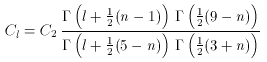
where Cl = < |alm|2. For such a
spectrum and correlation function, it can be shown that a power-law
initial density fluctuation spectrum, P(k)
if n < 3, l
which is the mean rms temperature fluctuation expected in the
quadrupole component of the anisotropy averaged over all cosmic
observers and obtained by fitting the correlation function by a flat
spectrum of fluctuations.
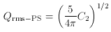
For the 4-year COBE DMR data, the best-fitting power spectrum of the
fluctuations has
n = 1.2 ± 0.3 and Qrms-PS =
15+4-3 µK
(Gorski et al.
1996),
although different analyses of the data by the
COBE team give slightly different errors and central values
(Wright et al.
1996;
Hinshaw et al.
1996).
These values are consistent with
the scale-invariant Harrison-Zel'dovich spectrum
(Harrison 1970;
Zel'dovich 1972;
Peebles & Yu 1970),
with n = 1 (P(k)


 . In that
case, the temperature field is
completely specified by the two-point correlation function
. In that
case, the temperature field is
completely specified by the two-point correlation function
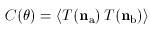
 = na
· nb
is the angle between the directions na
and nb. For a Gaussian random field,
= na
· nb
is the angle between the directions na
and nb. For a Gaussian random field,

 kn will produce
a spectrum with
kn will produce
a spectrum with
 2, and
the Sachs-Wolfe effect dominates the primordial fluctuations
(Bond & Efstathiou 1987). In this case, the
character of the fluctuations is usually described by the
best-fitting index n and
2, and
the Sachs-Wolfe effect dominates the primordial fluctuations
(Bond & Efstathiou 1987). In this case, the
character of the fluctuations is usually described by the
best-fitting index n and
 k), and
hence with the usual picture of random fluctuations growing to form
galaxies and clusters of galaxies following a phase of inflation
(Starobinsky 1980;
Guth 1981;
Bardeen et al. 1983).
k), and
hence with the usual picture of random fluctuations growing to form
galaxies and clusters of galaxies following a phase of inflation
(Starobinsky 1980;
Guth 1981;
Bardeen et al. 1983).
3 This, and all
later, limits have been converted to 1 from the 95 per cent
confidence limits quoted in the Fixsen et al. paper.
Back.
from the 95 per cent
confidence limits quoted in the Fixsen et al. paper.
Back.