


Consider a variable source which produces a variation that can be observed using more than one ray. As the travel time along these rays differs, the corresponding images will vary in brightness at different observing times. If the source is continuously variable, then we should be able to measure the time delay using cross-correlation techniques. The precision with which it can be measured depends on the amplitude and timescale of the source variability, on the frequency of observations and photometric accuracy, and on the value of the time delay itself.
Let us consider optical observations of quasars. Assuming that quasar variability is a stationary process, it can be described in terms of the first-order structure function:
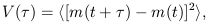
| (3.17) |
where m(t), m(t +
 ) are quasar magnitudes recorded at
two epochs separated by an
interval
(Simonetti, Cordes &
Heeschen 1985).
The qualifier "stationary" refers to the
assumption that V is not a function of the observation epoch
t, but only of the time lag
between two points on the light
curve. In practice, V() can
be well approximated by
a power law for time delays between a few days and a few years:
) are quasar magnitudes recorded at
two epochs separated by an
interval
(Simonetti, Cordes &
Heeschen 1985).
The qualifier "stationary" refers to the
assumption that V is not a function of the observation epoch
t, but only of the time lag
between two points on the light
curve. In practice, V() can
be well approximated by
a power law for time delays between a few days and a few years:

| (3.18) |
where the numerical coefficients were estimated from
Press, Rybicki &
Hewitt (1992a);
Cristiani et al. (1996);
and from the light curves of several lenses monitored at the Apache
Point Observatory. The amplitude of
V() depends on the bandpass
and it is larger at bluer wavelengths.
Equation 3.18 illustrates the difficulties associated with measuring
short time delays.
If the predicted delay is a few days, the expected amplitude of quasar
variations is
only ~ 0.02 magnitudes, requiring millimagnitude photometry in systems
that are often
complicated and marginally resolved from the ground (In quadruple
lenses, one has to
resolve four quasar images in a ~ 1" radius, superimposed on the diffuse
light of the
lensing galaxy). Even in a resolved system with a much longer time
delay, the double
quasar 0957+561, there has been much debate about the
correct value of
the delay, with estimates ranging from ~ 540 days
(Lehár et al. 1992;
Press et al. l992a,
1992b;
Beskin & Oknyanskij
1995)
to ~ 420 days
(Vanderriest et
al. 1989;
Schild & Cholfin 1986;
Schild & Thomson 1995;
Pelt et al. 1994,
1996).
Optical data recently acquired at
the Apache Point Observatory by Kundic et al.
(1995,
1997)
unambiguously measure a
delay of  t = 417 ±
3 days, vindicating the second group. This result required ~ 100
flux measurements in two observing seasons with a median photometric
error of < 1%.
t = 417 ±
3 days, vindicating the second group. This result required ~ 100
flux measurements in two observing seasons with a median photometric
error of < 1%.
A less accurate time delay of 12±3 days has been reported for the radio ring B0218+357 on the basis of radio polarization measurements (Corbett et al. 1996). The advantage of the polarization method over direct photometry is that only one parameter (time delay) is needed to align light curves of two images. Alignment of photometric light curves requires an additional parameter, corresponding to the relative magnification of the two images. More recently, Schechter et al. (1996) reported a measurement of two time delays in the quadruple quasar PG1115+080: 23.7 ± 3.4 days between images B and C and 9.4 days between images C and A. Unfortunately, it is not yet possible to model PG1115+080 accurately and so this impressive observation cannot furnish a useful estimate of the Hubble constant at this time. Sources like B1422+231 (Hjorth et al. 1996) and PKS1830-211 (van Ommen et al. 1995) are also currently being monitored.