4. MODELING STRONG GALAXY LENSES

4.1. The models

Any estimate of H₀ derived from gravitational lensing will be no better than the lens model that is deduced from observations of the positions and fluxes of the individual images. Lens modeling is, necessarily, a rather subjective business. The procedure that has to be followed depends upon whether or not the images are resolved. In most cases, there are N unresolved point images giving 2(N - 1) relative coordinates. There are also (N - 1) relative fluxes which can be fit to the magnification ratios. Since sources are variable, fluxes must be compared at the same emission time. (A complication that can arise at optical wavelengths is that individual stars in the lensing galaxy can cause additional, variable magnification, called microlensing, if the source is sufficiently compact. However, this is unlikely to be a problem at infrared or radio wavelengths.) So, with N point images, there are usually 3(N - 1) observables which can be used in model fitting. Once the relative time delays in the system are measured, they provide (N - 2) additional constraints.

Resolved images contain more information. Firstly, when compact radio sources are resolved using VLBI, the individual images ought to be related by a simple, four parameter, linear transformation (Eq. 2.16). This can be measured and is more useful than the flux ratio alone in constraining the model, and would give an additional 3(N - 1) observables. Secondly, if the radio structure is large enough, it is possible to expand to one higher order and measure the gradient of µ_ij. Thirdly, some sources are so extended that they form ring-like images. This can happen at either radio or optical wavelengths. In this case we have a large number, perhaps thousands of independent pixels to match up. In principle, this can lead to a highly constrained lens (and source) model. The best techniques for tackling this problem at radio wavelengths (Wallington, Kochanek & Narayan 1996) incorporate the model fitting as a stage in the map making procedure and, in some cases this can lead to impressively good models.

In order to model a simple gravitational lens, the scaled potential of the lensing galaxy, (plus any additional galaxies close enough to contribute to the deflection) is modeled using a simple function that contains adjustable parameters that measure the depth of the potential, its core radius, its ellipticity and its radial variation. A convenient functional form is the elliptical potential

(4.19)

where = (x, y) measures distance from the center of the potential which is located at (x₀, y₀). The two parameters _c, _s combine to describe the ellipticity and the position angle of the major axis. The exponent q measures the radial variation of the density at large radius. A value q = 0.5 corresponds to an isothermal sphere and a value q = 1 has asymptotically r^-2 as might be appropriate if, for example, mass traces light as in a Hubble profile. The elliptical potential has the advantage that it is quick to compute and good for searches in multi-dimensional parameter space. Its drawback is that the corresponding surface density is peanut-shaped at large ellipticity. Either two potentials must be superposed to generate realistic surface density distributions or a choice made from a smorgasbord of more complicated potentials (e.g. Schneider et al. 1992). In some cases, these potentials can be located and oriented using the observed galaxy image. However, we know that the mass in galaxies does not completely trace the light; in particular it diminishes more slowly with increasing radius. Therefore, we still have some freedom in modeling the mass distribution of lensing galaxies, even if their light profiles are well known. An example of the elliptical potential model is shown in Fig. 2. Motivated by the optical HST images of 1608+656, two elliptical potentials are superimposed to produce the observed quad configuration.

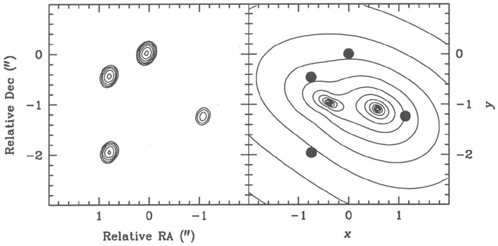
Figure 2. Radio map of the gravitational lens system 1608+656. The system was observed on 1996 October 10 with the VLA at 8.4 GHz. The map shows four unresolved images of the background source (at zs = 1.39). The brightest image (A) is located at the origin. (Courtesy of Chris Fassnacht.) Right: A simple model for 1608+656, consisting of two elliptical potentials. Solid lines represent logarithmically spaced density contours of the lensing mass distribution. The observed image positions (marked with dots) and their relative fluxes are accurately reproduced by this model.

It is also conventional to augment the lensing galaxy potential with a simple quadratic form,

(4.20)

which is trace-free and corresponds to a pure shear of the images. The external shear has two origins: dark matter lying in the lens plane associated with galaxies outside the strong lensing region and large-scale structure along the line of sight, as we discuss in more detail below.

A common procedure for modeling well observed gravitational lenses is to decide upon a list of independent observables and a smaller number of lens model parameters. These parameters are then varied so as to minimize some measure of the goodness of fit, typically a ² associated with the differences in the observables as predicted by the model from those actually measured. This approach has the merit of rewarding simplicity. However, the fit is usually somewhat imperfect and it is difficult to assign a formal error. A somewhat better approach, that is much harder to implement in practice, is to construct families of more elaborate models that may contain more parameters than observables and which are consequently underdetermined. Using this approach, it ought to be possible to derive many models that exactly recover the observables. We can then assign two types of error to the model time delay. One is associated with the measurement errors in the observables, the other depends upon the freedom in the models and it is here that the outcome depends most subjectively upon what we are prepared to countenance.

4.2. Modeling "quad" sources

Let us describe some of the dangers and possibilities involved in model fitting by considering image formation in a simple case, the so-called "quad" sources. These are quadruply imaged point sources formed by a galaxy for which the circular symmetry is broken by an elliptical perturbation. (Depending upon the nature of the potential in the galaxy nucleus, there may also be a fifth, faint, central image which we shall ignore.) For illustration, we use the simplest possible model of a singular isothermal sphere potential perturbed by a quadratic shear, and work to first order in the ellipticity (cf Blandford & Kovner 1988).

We write the potential in the form

(4.21)

where polar coordinates = (, ) refer to the center of the potential located at the center of the observed lensing galaxy (Fig. 3). The first term ⁰_s = ₀ describes an isothermal sphere ( ^-1), and is circularly symmetric. The second term is the non-circular perturbation. We assume that we know its orientation from the shape of the galaxy but treat the ellipticity as unknown. If we set = 0 and place a source on the axis, then the image will be a circular ring of radius ₀ known as the Einstein ring. We now switch on the perturbation and solve for the source position to linear order assuming that << 1. We find that the source position is

(4.22)

where = - ₀, and , are unit vectors in the radial and tangential directions respectively. We can now evaluate the Hessian and find that its eigenvalues are

(4.23)

and the principal axes are rotated with respect to , by an angle

(4.24)

These eigenvalues are the reciprocals of the quasi-radial and quasi-tangential magnifications, so that the total magnification is µ = (h₁ h₂)^-1 = ( / ₀ - cos 2)^-1. The locus of the infinite magnification on the sky, the "critical curve" is then given by h₂ = 0 or

(4.25)

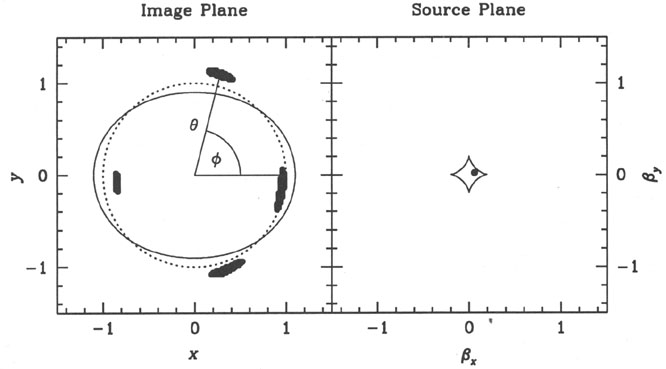
The critical curve is the image of the "caustic", the locus in the source plane of points that are infinitely magnified. Its equation is

(4.26)

which is the parametric equation of an astroid. If we know the source position, , and it is located within the astroid then there will be four images located close to the critical curve (Fig. 3). If the source lies outside the astroid, there will be two images.

Figure 3. Lensing geometry giving rise to a four-image ("quad") configuration. If the source is located within the astroid (diamond) caustic produced by an elliptical potential (right panel), there will be four tangentially elongated images near the critical curve (solid line) in the image plane (left panel). Dotted line in the left panel corresponds to the Einstein ring of the unperturbed, circularly symmetric lens.

This model has two free parameters, and ₀, and as we may have eleven observables in a four-image lens (three pairs of relative positions + three flux ratios + two time delay ratios), there are many internal consistency checks. For example, the angles of the four images must satisfy

(4.27)

Now, in order to trust the model, we contend that it is necessary that every observable be fit within its measurement error, or there should be a good reason why it can be excused. For example, we might have a spectroscopic indication that microlensing is at work in one of the images and then we would discount the measurement of its flux.

Now, it is extremely unlikely that any lens will ever be found that is this simple. So, after we are sure that there is inconsistency, we must introduce additional parameters or change the model. Following the above approach of expanding about the Einstein ring, we can (or may have to) allow the center of the potential to vary, adjust the orientation of the perturbations, allow the ellipticity to vary with radius , introduce higher harmonics (e.g. cos 4 for box-like equipotentials) and so on. Alternatively, we can turn to a density-based model. The nature and quality of the observations will usually dictate this choice.

What we discover when we carry out this procedure is that the allowed range of observables is quite sensitive not just to the parameters, but to the functional form of the model. For example, constraint 4.27 is quite general but can be violated if (not unreasonably) we were to add a cos 4 term. In addition, the shape of the unperturbed, circular potential controls the quasi-radial magnification and changing it changes h₁ to 1 - d^{2 0}_s / d². The ratios of time lags are fairly well fixed by the observed image magnifications and location; however, the absolute values (in which we are primarily interested) are extremely sensitive to radial variation of the ellipticity and this can be measured if we have very accurate image positions or an extended source. Finally, we should probably always include the quadratic form Eq. 4.20 to take account of distant mass.

There are further possible consistency checks. For example, if we can make VLBI observations of the individual image components, as should be possible for 1608+656 (Myers et al. 1995, Fassnacht et al. 1996; Fig. 2), and resolve structure in the radial direction, we can also check both the radial eigenvalue h₁, and the orientation angle for each of the images. Even better, if we have more than one source, as appears to be the case in 1933+503 (Sykes et al. 1996), than we have two independent opportunities to test the model and derive the parameters. (This approach may also be of interest for cluster arcs.)

Let us use the quad H1413+117 for illustration and try to model it using a simple potential (Eq. 4.21). We can guess the lens center pretty accurately, but not the position angle of the major axis of the elliptical perturbation, ₀. Using Eq. 4.27, we find four choices for ₀ and we examine each of these in turn to try to find a consistent solution for the source position by varying , ₀, and the lens center. We find that none of our choices of ₀ can accomplish this, although one comes close. However, if we now compute the magnification ratios, we find that they are quite inconsistent with the observations. Therefore we can assuredly reject our lens model. It turns out that it is possible to reproduce the positions and fluxes using an elliptical potential with parameters {b, s, q, _c, _s, x_c, y_c} offset by an external shear with parameters _c, _s. Although this seems the most plausible model, it is not unique (Yun et al. 1996, preprint) and this would be a concern were this a good choice for monitoring. Unfortunately, it is not as the predicted time delays are almost certainly too small.

4.3. Uncertainties in the models

An important question that we must now address is "How do we assign a formal error to the predicted model on the basis of a deflector model?" One procedure is to define a ² using careful values for the measurement errors and then choose parameters p_i that minimize this statistic. We then compute a covariance matrix

(4.28)

and invert and diagonalize this quantity so as to form the error ellipsoid. We next compute the maximum fractional change in the time delay within this error ellipsoid and quote this as the fractional error in the derived Hubble constant varying the parameters independently until ² / increases by unity. The maximum change in the derived value of the delay as we go through this procedure is the required error in the delay.

However, this is still not enough because existence does not imply uniqueness. Suppose that we have a model that truly reproduces all the observables giving an acceptable value for ² and for which the underlying mass distribution is dynamically possible. We should still aggressively explore all other classes of models that can also fit the observations but yet which produce disjoint estimates for the time delay. The true uncertainty in the Hubble constant is given by the union of all of these models. This is a large task. Clearly, we may have to introduce some practical limitations. It is probably quite safe to reject dynamically unreasonable mass distributions, for example positive radial gradients in surface density, but are we allowed to posit isolated concentrations of unseen mass? Of course, only time will tell whether there are genuinely dark galaxies, but until we can demonstrate that all significant perturbers are luminous we must allow for this possibility. There is already an indication that there may be more unseen mass than we have already included in the discovery that the incidence of quad sources relative to doubles is much greater than one might have expected if the lenses are about as elliptical as normal galaxies (King & Browne 1996). Three explanations have been advanced for this discrepancy. Firstly, the total mass associated with the observed lensing galaxies may be highly elliptical, or, indeed, quite irregular. (It appears that observed faint galaxies have a median ellipticity of ~ 0.4 as opposed to ~ 0.15 for local galaxies.) Secondly, many of the lenses may actually have unseen companions so that the combined potential will generally be quite elliptical. Thirdly, as we discuss below, propagation effects associated dark matter long the line of sight may actually promote the formation of quads.

4.4. The double quasar 0957+561

We now briefly turn from quads to the important case of 0957+561, the only gravitational lens where the time delay has been measured with high accuracy (Kundic et al. 1997). Traditionally, 0957+561 was thought to be a difficult system to model because of the small number of constraints in its two-image configuration and because of the complexity of the lensing potential - the primary lensing galaxy G1 is surrounded by a cluster. To a large extent, these problems have been resolved in the extensive theoretical study of Grogin & Narayan (1996). The crucial set of constraints in the GN model was provided by high spatial resolution VLBI mapping of Garrett et al. (1994), which resolved inner jets in both images of the source into five centers of emission. Mapping of one jet into the other fixed the relative magnification tensor of images A and B (Eq. 2.16), as well as its gradients along and perpendicular to the jet. This, in turn, provided a tight constraint on the radial mass profile (dM / dr) at the image locations, which, together with the total enclosed mass M(< r), controls the conversion factor between the time delay and the physical distance to the lens. The importance of the dM / dr term was nicely illustrated by Wambsganss & Paczynski (1994).

The remaining model degeneracy in the 0957+561 system between the lensing galaxy G1 and its host cluster cannot be removed by using relative image positions and magnifications (Falco, Gorenstein & Shapiro 1985). It has to be broken by either directly measuring the mass of G1 via its velocity dispersion, or by measuring the surface density in the cluster from its weak shearing effect on the images of background galaxies (e.g. Tyson, Valdes & Wenk 1990, Kaiser & Squires 1993). If both of these parameters are independently determined, they provide an important consistency check on the model.

Falco et al. (1996, private communication) recently observed G1 with the LRIS spectrograph at the Keck. Their high signal-to-noise spectrum yields a line-of-sight velocity dispersion roughly in the range _obs = 275 ± 30 km/s (2), consistent with the only published measurement by Rhee (1991), _obs = 303 ± 50 km/s. Using a deep CFHT image of the field, Fischer et al. (1997) mapped the cluster mass distribution from the distortion of faint background galaxies. Adopting their estimate of the mean background galaxy redshift (z_b = 1.2) gives the dimensionless cluster surface mass density = / _c = 0.18±0.11 (2). Using these two results and their measurement of the time delay, Kundic et al. (1997) find

(4.29)   (4.30)

The uncertainty in H₀ is quoted at 2 and allows for finite aperture effects and anisotropy of stellar orbits in conversion of _obs to G1 mass (GN). While this estimate of H₀ can certainly be improved by future observations, it is already 10% accurate at the 1 level.