3. PHYSICS OF TEMPERATURE FLUCTUATIONS

The minute temperature fluctuations present in the microwave background contain a wealth of information about the fundamental properties of the universe. In order to understand the reasons for this and the kinds of information available, an appreciation of the underlying physical processes generating temperature and polarization fluctuations is required. This section and the following one give a general description of all basic physics processes involved in producing microwave background fluctuations.

First, one practical matter. Throughout these lectures, common cosmological units will be employed in which = c = k_b = 1. All dimensionful quantities can then be expressed as powers of an energy scale, commonly taken as GeV. In particular, length and time both have units of [GeV]^-1, while Newton's constant G has units of [GeV]^-2 since it is defined as equal to the square of the inverse Planck mass. These units are very convenient for cosmology, because many problems deal with widely varying scales simultaneously. For example, any computation of relic particle abundances (e.g. primordial nucleosynthesis) involves both a quantum mechanical scale (the interaction cross-section) and a cosmological scale (the time scale for the expansion of the universe). Conversion between these cosmological units and physical (cgs) units can be achieved by inserting needed factors of , c, and k_b. The standard textbook by Kolb and Turner (1990) contains an extremely useful appendix on units.

3.1. Causes of temperature fluctuations

Blackbody radiation in a perfectly homogeneous and isotropic universe, which is always adopted as a zeroth-order approximation, must be at a uniform temperature, by assumption. When perturbations are introduced, three elementary physical processes can produce a shift in the apparent blackbody temperature of the radiation emitted from a particular point in space. All temperature fluctuations in the microwave background are due to one of the following three effects.

The first is simply a change in the intrinsic temperature of the radiation at a given point in space. This will occur if the radiation density increases via adiabatic compression, just as with the behavior of an ideal gas. The fractional temperature perturbation in the radiation just equals the fractional density perturbation.

The second is equally simple: a doppler shift if the radiation at a particular point is moving with respect to the observer. Any density perturbations within the horizon scale will necessarily be accompanied by velocity perturbations. The induced temperature perturbation in the radiation equals the peculiar velocity (in units of c, of course), with motion towards the observer corresponding to a positive temperature perturbation.

The third is a bit more subtle: a difference in gravitational potential between a particular point in space and an observer will result in a temperature shift of the radiation propagating between the point and the observer due to gravitational redshifting. This is known as the Sachs-Wolfe effect, after the original paper describing it (Sachs and Wolfe, 1967). This paper contains a completely straightforward general relativistic calculation of the effect, but the details are lengthy and complicated. A far simpler and more intuitive derivation has been given by Hu and White (1997) making use of gauge transformations. The Sachs-Wolfe effect is often broken into two pieces, the usual effect and the so-called Integrated Sachs-Wolfe effect. The latter arises when gravitational potentials are evolving with time: radiation propagates into a potential well, gaining energy and blueshifting in the process. As it climbs out, it loses energy and redshifts, but if the depth of the potential well has increased during the time the radiation propagates through it, the redshift on exiting will be larger than the blueshift on entering, and the radiation will gain a net redshift, appearing cooler than it started out. Gravitational potentials remain constant in time in a matter-dominated universe, so to the extent the universe is matter dominated during the time the microwave background radiation freely propagates, the Integrated Sachs-Wolfe effect is zero. In models with significantly less than critical density in matter (i.e. the currently popular CDM models), the redshift of matter-radiation equality occurs late enough that the gravitational potentials are still evolving significantly when the microwave background radiation decouples, leading to a non-negligible Integrated Sachs-Wolfe effect. The same situation also occurs at late times in these models; gravitational potentials begin to evolve again as the universe makes a transition from matter domination to either vacuum energy domination or a significantly curved background spatial metric, giving an additional Integrated Sachs-Wolfe contribution.

3.2. A formal description

The early universe at the epoch when the microwave background radiation begins propagating freely, around a redshift of z = 1100, is a conceptually simple place. Its constituents are ``baryons'' (including protons, helium nuclei, and electrons, even though electrons are not baryons), neutrinos, photons, and dark matter particles. The neutrinos and dark matter can be treated as interacting only gravitationally since their weak interaction cross-sections are too small at this energy scale to be dynamically or thermodynamically relevant. The photons and baryons interact electromagnetically, primarily via Compton scattering of the radiation from the electrons. The typical interaction energies are low enough for the scattering to be well-approximated by the simple Thomson cross section. All other scattering processes (e.g. Thomson scattering from protons, Rayleigh scattering of radiation from neutral hydrogen) have small enough cross-sections to be insignificant, so we have four species of matter with only one relevant (and simple) interaction process among them. The universe is also very close to being homogeneous and isotropic, with small perturbations in density and velocity on the order of a part in 10⁵. The tiny size of the perturbations guarantees that linear perturbation theory around a homogeneous and isotropic background universe will be an excellent approximation.

Conceptually, the formal description of the universe at this epoch is quite simple. The unperturbed background cosmology is described by the Friedmann-Robertson-Walker (FRW) metric, and the evolution of the cosmological scale factor a(t) in this metric is given by the Friedmann equation (see the lectures by Peacock in this volume). The evolution of the free electron density n_e is determined by the detailed atomic physics describing the recombination of neutral hydrogen and helium; see Seager et al. (2000) for a detailed discussion. At a temperature of around 0.5 eV, the electrons combine with the protons and helium nuclei to make neutral atoms. As a result, the photons cease Thomson scattering and propagate freely to us. The microwave background is essentially an image of the ``surface of last scattering''. Recombination must be calculated quite precisely because the temperature and thickness of this surface depend sensitively on the ionization history through the recombination process.

The evolution of first-order perturbations in the various energy density components and the metric are described with the following sets of equations:

• The photons and neutrinos are described by distribution functions f (x, p, t). A fundamental simplifying assumption is that the energy dependence of both is given by the blackbody distribution. The space dependence is generally Fourier transformed, so the distribution functions can be written as (k, , t), where the function has been normalized to the temperature of the blackbody distribution and represents the direction in which the radiation propagates. The time evolution of each is given by the Boltzmann equation. For neutrinos, collisions are unimportant so the Boltzmann collision term on the right side is zero; for photons, Thomson scattering off electrons must be included.

• The dark matter and baryons are in principle described by Boltzmann equations as well, but a fluid description incorporating only the lowest two velocity moments of the distribution functions is adequate. Thus each is described by the Euler and continuity equations for their densities and velocities. The baryon Euler equation must include the coupling to photons via Thomson scattering.

• Metric perturbation evolution and the connection of the metric perturbations to the matter perturbations are both contained in the Einstein equations. This is where the subtleties arise. A general metric perturbation has 10 degrees of freedom, but four of these are unphysical gauge modes. The physical perturbations include two degrees of freedom constructed from scalar functions, two from a vector, and two remaining tensor perturbations (Mukhanov et al. 1992). Physically, the scalar perturbations correspond to gravitational potential and anisotropic stress perturbations; the vector perturbations correspond to vorticity and shear perturbations; and the tensor perturbations are two polarizations of gravitational radiation. Tensor and vector perturbations do not couple to matter evolving only under gravitation; in the absence of a ``stiff source'' of stress energy, like cosmic defects or magnetic fields, the tensor and vector perturbations decouple from the linear perturbations in the matter.

A variety of different variable choices and methods for eliminating the gauge freedom have been developed. The subject can be fairly complicated. A detailed discussion and comparison between the Newtonian and synchronous gauges, along with a complete set of equations, can be found in Ma and Bertschinger (1995); also see Hu et al. (1998). An elegant and physically appealing formalism based on an entirely covariant and gauge-invariant description of all physical quantities has been developed for the microwave background by Challinor and Lasenby (1999) and Gebbie et al. (2000), based on earlier work by Ehlers (1993) and Ellis and Bruni (1989). A more conventional gauge-invariant approach was originated by Bardeen (1980) and developed by Kodama and Sasaki (1984).

The Boltzmann equations are partial differential equations, which can be converted to hierarchies of ordinary differential equations by expanding their directional dependence in Legendre polynomials. The result is a large set of coupled, first-order linear ordinary differential equations which form a well-posed initial value problem. Initial conditions must be specified. Generally they are taken to be so-called adiabatic perturbations: initial curvature perturbations with equal fractional perturbations in each matter species. Such perturbations arise naturally from the simplest inflationary scenarios. Alternatively, isocurvature perturbations can also be considered: these initial conditions have fractional density perturbations in two or more matter species whose total spatial curvature perturbation cancels. The issue of numerically determining initial conditions is discussed below in Sec. 5.2.

The set of equations are numerically stiff before last scattering, since they contain the two widely discrepant time scales: the Thomson scattering time for electrons and photons, and the (much longer) Hubble time. Initial conditions must be set with high accuracy and an appropriate stiff integrator must be employed. A variety of numerical techniques have been developed for evolving the equations. Particularly important is the line-of-sight algorithm first developed by Seljak and Zaldarriaga (1996) and then implemented by them in the publicly-available CMBFAST code
(see http://www.sns.ias.edu/~matiasz/CMBFAST/cmbfast.html).

The above discussion is intentionally heuristic and somewhat vague because many of the issues involved are technical and not particularly illuminating. My main point is an appreciation for the detailed and precise physics which goes into computing microwave background fluctuations. However, all of this formalism should not obscure several basic physical processes which determine the ultimate form of the fluctuations. A widespread understanding of most of the physical processes detailed below followed from a seminal paper by Hu and Sugiyama (1996), a classic of the microwave background literature.

3.3. Tight coupling

Two basic time scales enter into the evolution of the microwave background. The first is the photon scattering time scale t_s, the mean time between Thomson scatterings. The other is the expansion time scale of the universe, H^-1, where H = / a is the Hubble parameter. At temperatures significantly greater than 0.5 eV, hydrogen and helium are completely ionized and t_s << H^-1. The Thomson scatterings which couple the electrons and photons occur much more rapidly than the expansion of the universe; as a result, the baryons and photons behave as a single ``tightly coupled'' fluid. During this period, the fluctuations in the photons mirror the fluctuations in the baryons. (Note that recombination occurs at around 0.5 eV rather than 13.6 eV because of the huge photon-baryon ratio; the universe contains somewhere around 10⁹ photons for each baryon, as we know from primordial nucleosynthesis. It is a useful exercise to work out the approximate recombination temperature.)

The photon distribution function for scalar perturbations can be written as (k, µ, t) where µ = . and the scalar character of the fluctuations guarantees the distribution cannot have any azimuthal directional dependence. (The azimuthal dependence for vector and tensor perturbations can also be included in a similar decomposition). The moments of the distribution are defined as

(1)

sometimes other normalizations are used. Tight coupling implies that _l = 0 for l > 1. Physically, the l = 0 moment corresponds to the photon energy density perturbation, while l = 1 corresponds to the bulk velocity. During tight coupling, these two moments must match the baryon density and velocity perturbations. Any higher moments rapidly decay due to the isotropizing effect of Thomson scattering; this follows immediately from the photon Boltzmann equation.

3.4. Free streaming

In the other regime, for temperatures significantly lower than 0.5 eV, t_s >> H^-1 and photons on average never scatter again until the present time. This is known as the ``free streaming'' epoch. Since the radiation is no longer tightly coupled to the electrons, all higher moments in the radiation field develop as the photons propagate. In a flat background spacetime, the exact solution is simple to derive. After scattering ceases, the photons evolve according to the Liouville equation

(2)

with the trivial solution

(3)

where we have converted to conformal time defined by d = dt / a(t) and _* corresponds to the time at which free streaming begins. Taking moments of both sides results in

(4)

with j_l a spherical Bessel function. The process of free streaming essentially maps spatial variations in the photon distribution at the last scattering surface (wavenumber k) into angular variations on the sky today (moment l).

3.5. Diffusion damping

In the intermediate regime during recombination, t_s H^-1. Photons propagate a characteristic distance L_D during this time. Since some scattering is still occurring, baryons experience a drag from the photons as long as the ionization fraction is appreciable. A second-order perturbation analysis shows that the result is damping of baryon fluctuations on scales below L_D, known as Silk damping or diffusion damping. This effect can be modelled by the replacement

(5)

although detailed calculations are needed to define L_D precisely. As a result of this damping, microwave background fluctuations are exponentially suppressed on angular scales significantly smaller than a degree.

3.6. The resulting power spectrum

The fluctuations in the universe are assumed to arise from some random statistical process. We are not interested in the exact pattern of fluctuations we see from our vantage point, since this is only a single realization of the process. Rather, a theory of cosmology predicts an underlying distribution, of which our visible sky is a single statistical realization. The most basic statistic describing fluctuations is their power spectrum. A temperature map on the sky T() is conventionally expanded in spherical harmonics,

(6)

where

(7)

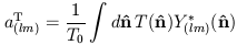
are the temperature multipole coefficients and T₀ is the mean CMB temperature. The l = 1 term in Eq. (6) is indistinguishable from the kinematic dipole and is normally ignored. The temperature angular power spectrum C_l is then given by

(8)

where the angled brackets represent an average over statistical realizations of the underlying distribution. Since we have only a single sky to observe, an unbiased estimator of C_l is constructed as

(9)

The statistical uncertainty in estimating C^T_l by a sum of 2l + 1 terms is known as ``cosmic variance''. The constraints l = l' and m = m' follow from the assumption of statistical isotropy: C^T_l must be independent of the orientation of the coordinate system used for the harmonic expansion. These conditions can be verified via an explicit rotation of the coordinate system.

A given cosmological theory will predict C^T_l as a function of l, which can be obtained from evolving the temperature distribution function as described above. This prediction can then be compared with data from measured temperature differences on the sky. Figure 1 shows a typical temperature power spectrum from the inflationary class of models, described in more detail below. The distinctive sequence of peaks arise from coherent acoustic oscillations in the fluid during the tight coupling epoch and are of great importance in precision tests of cosmological models; these peaks will be discussed in Sec. 5. The effect of diffusion damping is clearly visible in the decreasing power above l = 1000. When viewing angular power spectrum plots in multipole space, keep in mind that l = 200 corresponds approximately to fluctuations on angular scales of a degree, and the angular scale is inversely proportional to l. The vertical axis is conventionally plotted as l (l + 1)C^T_l because the Sachs-Wolfe temperature fluctuations from a scale-invariant spectrum of density perturbations appears as a horizontal line on such a plot.

Figure 1. The temperature angular power spectrum for a cosmological model with mass density 0 = 0.3, vacuum energy density = 0.7, Hubble parameter h = 0.7, and a scale-invariant spectrum of primordial adiabatic perturbations.