5. ACOUSTIC OSCILLATIONS

Before decoupling, the matter in the universe has significant pressure because it is tightly coupled to radiation. This pressure counteracts any tendency for matter to collapse gravitationally. Formally, the Jeans mass is greater than the mass within a horizon volume for times earlier than decoupling. During this epoch, density perturbations will set up standing acoustic waves in the plasma. Under certain conditions, these waves leave a distinctive imprint on the power spectrum of the microwave background, which in turn provides the basis for precision constraints on cosmological parameters. This section reviews the basics of the acoustic oscillations.

5.1. An oscillator equation

In their classic 1996 paper, Hu and Sugiyama transformed the basic equations describing the evolution of perturbations into an oscillator equation. Combining the zeroth moment of the photon Boltzmann equation with the baryon Euler equation for a given k-mode in the tight-coupling approximation (mean baryon velocity equals mean radiation velocity) gives

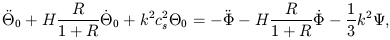
(27)

where ₀ is the zeroth moment of the temperature distribution function (proportional to the photon density perturbation), R = 3_b / 4 is proportional to the scale factor a, H = / a is the conformal Hubble parameter, and the sound speed is given by c_s² = 1 / (3 + 3R). (All overdots are derivatives with respect to conformal time.) and are the scalar metric perturbations in the Newtonian gauge; if we neglect the anisotropic stress, which is generally small in conventional cosmological scenarios, then = - . But the details are not very important. The equation represents damped, driven oscillations of the radiation density, and the various physical effects are easily identified. The second term on the left side is the damping of oscillations due to the expansion of the universe. The third term on the left side is the restoring force due to the pressure, since c_s² = dP / d. On the right side, the first two terms depend on the time variation of the gravitational potentials, so these two are the source of the Integrated Sachs-Wolfe effect. The final term on the right side is the driving term due to the gravitational potential perturbations. As Hu and Sugiyama emphasized, these damped, driven acoustic oscillations account for all of the structure in the microwave background power spectrum.

A WKB approximation to the homogeneous equation with no driving source terms gives the two oscillation modes (Hu and Sugiyama 1996)

(28)

where the sound horizon r_s is given by

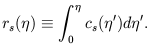
(29)

Note that at times well before matter-radiation equality, the sound speed is essentially constant, c_s = 1 / 3, and the sound horizon is simply proportional to the causal horizon. In general, any perturbation with wavenumber k will set up an oscillatory behavior in the primordial plasma described by a linear combination of the two modes in Eq. (28). The relative contribution of the modes will be determined by the initial conditions describing the perturbation.

Equation (27) appears to be simpler than it actually is, because and are the total gravitational potentials due to all matter and radiation, including the photons which the left side is describing. In other words, the right side of the equation contains an implicit dependence on ₀. At the expense of pedagogical transparency, this situation can be remedied by considering separately the potential from the photon-baryon fluid and the potential from the truly external sources, the dark matter and neutrinos. This split has been performed by Hu and White (1996). The resulting equation, while still an oscillator equation, is much more complicated, but must be used for a careful physical analysis of acoustic oscillations.

5.2. Initial conditions

The initial conditions for radiation perturbations for a given wavenumber k can be broken into two categories, according to whether the gravitational potential perturbation from the baryon-photon fluid, _b, is nonzero or zero as -> 0. The former case is known as ``adiabatic'' (which is somewhat of a misnomer since adiabatic technically refers to a property of a time-dependent process) and implies that n_b / n, the ratio of baryon to photon number densities, is a constant in space. This case must couple to the cosine oscillation mode since it requires ₀ 0 as -> 0. The simplest (i.e. single-field) models of inflation produce perturbations with adiabatic initial conditions.

The other case is termed ``isocurvature'' since the fluid gravitational potential perturbation _b, and hence the perturbations to the spatial curvature, are zero. In order to arrange such a perturbation, the baryon and photon densities must vary in such a way that they compensate each other: n_b / n varies, and thus these perturbations are in entropy, not curvature. At an early enough time, the temperature perturbation in a given k mode must arise entirely from the Sachs-Wolfe effect, and thus isocurvature perturbations couple to the sine oscillation mode. These perturbations arise from causal processes like phase transitions: a phase transition cannot change the energy density of the universe from point to point, but it can alter the relative entropy between various types of matter depending on the values of the fields involved. The potentially most interesting cause of isocurvature perturbations is multiple dynamical fields in inflation. The fields will exchange energy during inflation, and the field values will vary stochastically between different points in space at the end of the phase transition, generically giving isocurvature along with adiabatic perturbations (Polarski and Starobinsky 1994).

The numerical problem of setting initial conditions is somewhat tricky. The general problem of evolving perturbations involves linear evolution equations for around a dozen variables, outlined in Sec. 3.2. Setting the correct initial conditions involves specifying the value of each variable in the limit as -> 0. This is difficult for two reasons: the equations are singular in this limit, and the equations become increasingly numerically stiff in this limit. Simply using the leading-order asymptotic behavior for all of the variables is only valid in the high-temperature limit. Since the equations are stiff, small departures from this limiting behavior in any of the variables can lead to numerical instability until the equations evolve to a stiff solution, and this numerical solution does not necessarily correspond to the desired initial conditions. Numerical techniques for setting the initial conditions to high accuracy at temperaturesare currently being developed.

5.3. Coherent oscillations

The characteristic ``acoustic peaks'' which appear in Figure 1 arise from acoustic oscillations which are phase coherent: at some point in time, the phases of all of the acoustic oscillations were the same. This requires the same initial condition for all k-modes, including those with wavelengths longer than the horizon. Such a condition arises naturally for inflationary models, but is very hard to reproduce in models producing perturbations causally on scales smaller than the horizon. Defect models, for example, produce acoustic oscillations, but the oscillations generically have incoherent phases and thus display no peak structure in their power spectrum (Seljak et al. 1997). Simple models of inflation which produce only adiabatic perturbations insure that all perturbations have the same phase at = 0 because all of the perturbations are in the cosine mode of Eq. (28).

A glance at the k dependence of the adiabatic perturbation mode reveals how the coherent peaks are produced. The microwave background images the radiation density at a fixed time; as a function of k, the density varies like cos(kr_s), where r_s is fixed. Physically, on scales much larger than the horizon at decoupling, a perturbation mode has not had enough time to evolve. At a particular smaller scale, the perturbation mode evolves to its maximum density in potential wells, at which point decoupling occurs. This is the scale reflected in the first acoustic peak in the power spectrum. Likewise, at a particular still smaller scale, the perturbation mode evolves to its maximum density in potential wells and then turns around, evolving to its minimum density in potential wells; at that point, decoupling occurs. This scale corresponds to that of the second acoustic peak. (Since the power spectrum is the square of the temperature fluctuation, both compressions and rarefactions in potential wells correspond to peaks in the power spectrum.) Each successive peak represents successive oscillations, with the scales of odd-numbered peaks corresponding to those perturbation scales which have ended up compressed in potential wells at the time of decoupling, while the even-numbered peaks correspond to the perturbation scales which are rarefied in potential wells at decoupling. If the perturbations are not phase coherent, then the phase of a given k-mode at decoupling is not well defined, and the power spectrum just reflects some mean fluctuation power at that scale.

In practice, two additional effects must be considered: a given scale in k-space is mapped to a range of l-values; and radiation velocities as well as densities contribute to the power spectrum. The first effect broadens out the peaks, while the second fills in the valleys between the peaks since the velocity extrema will be exactly out of phase with the density extrema. The amplitudes of the peaks in the power spectrum are also suppressed by Silk damping, as mentioned in Sec. 3.5.

5.4. The effect of baryons

The mass of the baryons creates a distinctive signature in the acoustic oscillations (Hu and Sugiyama 1996). The zero-point of the oscillations is obtained by setting ₀ constant in Eq. (27): the result is

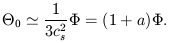
(30)

The photon temperature ₀ is not itself observable, but must be combined with the gravitational redshift to form the ``apparent temperature'' ₀ - , which oscillates around a. If the oscillation amplitude is much larger than a = 3_b / 4, then the oscillations are effectively about the mean temperature. The positive and negative oscillations are of the same amplitude, so when the apparent temperature is squared to form the power spectrum, all of the peaks have the same height. On the other hand, if the baryons contribute a significant mass so that a is a significant fraction of the oscillation amplitude, then the zero point of the oscillations are displaced, and when the apparent temperature is squared to form the power spectrum, the peaks arising from the positive oscillations are higher than the peaks from the negative oscillations. If a is larger than the amplitude of the oscillations, then the power spectrum peaks corresponding to the negative oscillations disappear entirely. The physical interpretation of this effect is that the baryon mass deepens the potential well in which the baryons are oscillating, increasing the compression of the plasma compared to the case with less baryon mass. In short, as the baryon density increases, the power spectrum peaks corresponding to compressions in potential wells get higher, while the alternating peaks corresponding to rarefactions get lower. This alternating peak height signature is a distinctive signature of baryon mass, and allows the precise determination of the cosmological baryon density with the measurement of the first several acoustic peak heights.