Using the CMB for Ho - A.N. Lasenby & M.E. Jones

2. THE SZ EFFECT

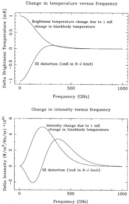
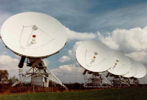
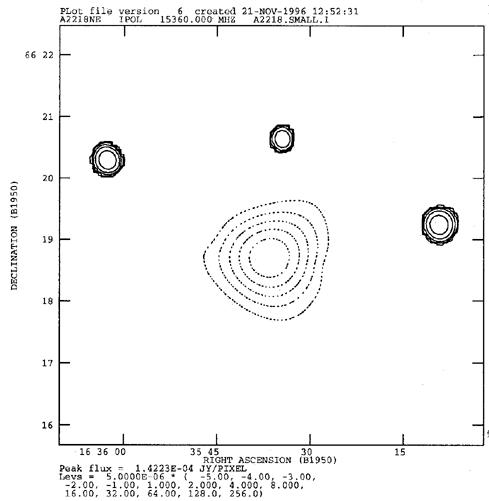
The basic mechanism of the SZ effect is a differential scattering to higher energies which occurs when photons from the CMB (Cosmic Microwave Background) pass through the hot gas of a cluster of galaxies (Sunyaev & Zel'dovich 1972). This results in a dip in the Rayleigh-Jeans region of the spectrum, and a corresponding increase in the Wien region (See Fig. 1). The effect was probably first reliably detected in the single-dish Owens Valley measurements of Birkinshaw et al. (1984) and has since been measured in detail for a variety of clusters by the Ryle Telescope in Cambridge (e.g. Jones et al. (1993), Grainge et al. (1993), Saunders (in press)), the Owens Valley interferometer (Carlstrom et al. 1996), the 5.5-m Owens Valley telescope (Herbig et al. 1995) and by the SuZie bolometer mounted at the Caltech Submillimeter Observatory, Hawaii (Wilbanks et al. 1994). The Ryle Telescope (see Fig. 2) has successfully provided maps of the effect for several clusters. A sample map of the SZ effect, in the cluster A2218, is given in Fig. 3.

Figure 1. The frequency dependences of the thermal and kinetic SZ effects expressed as a brightness temperature change (top) and intensity change (bottom).

Figure 2. The Ryle Telescope

Figure 3. Maximum-entropy deconvolved image of the cluster A2218 made with the Ryle Telescope. The three unresolved sources are not connected with the cluster. The central flux decrement is 500 ± 70µJy beam^-1, corresponding to a temperature decrement of 0.9^+0.06_-0.14 mK.

The way in which the SZ effect can be used to determine H₀ in conjunction with X-ray information is worth discussing in detail. We start with the equation for the X-ray flux:

where n_e and T_e are the electron number density and temperature, and D_L the luminosity distance to the cluster. Via the X-ray and optical information we can determine T_e, and z, where is a characteristic angular size of the cluster and z is the cluster redshift. The SZ effect is determined by

i.e. a line of sight integral of pressure through the cluster and we can relate dl to the other quantities via

Here f is a prolateness factor, which assuming the cluster has an ellipsoidal shape, is the ratio of the length of the major axis of the ellipse to the minor axis. The last equation uses the angular diameter distance formula to get the physical width of the cluster given its angular diameter, and then converts this to a line of sight distance through the cluster using this assumed prolateness. This is done assuming what will turn out to be a `worst case,' where the cluster is indeed prolate and pointing straight at the observer. If we assume the cluster is at not too high a redshift, then the luminosity distance can be approximated by D_L = cz / H₀ (Obviously more accurate formulae can be used for this and other quantities at higher redshift. We are just trying to give a schematic outline of the method). Eliminating n_e via the known S_X, and D_L in favor of H₀, one finds

with the constant of proportionality known. We note straightaway that if f is assumed to be 1 when it is really > 1, i.e. where the cluster is indeed oriented towards the observer, then the H₀ derived by this method will come out too small. Since the H₀'s found so far using this approach have tended to come out lower than optical determinations, it is obviously this case that we need to worry about most in the first instance. Furthermore for clusters which are selected on the basis of X-ray surface brightness, there would be a tendency for just this effect to happen, since the greater line of sight distance through the cluster would emphasize their X-ray brightness.

Putting back further factors we get

(2.1)

T_e can be found from the X-ray spectrum obtained e.g. with the GINGA or ASCA satellites, which cover the range up to ~ 10 keV. A typical cluster temperature is T_e ~ 6 keV and ROSAT only covers the range up to ~ 2 keV. The X-ray flux, S_X, can be obtained from e.g. ASCA, with resolution ~ 2', or the ROSAT PSPC, with resolution ~ 15". The cluster profile is modeled generally via an assumed isothermal atmosphere, with

Typical values for clusters are beta ~ 0.6, and core radius r_c ~ 0.25 Mpc, but one has to fit for these in any given case. For elliptical clusters, Grainge (1996) has described how one can allow for different core radii along orthogonal axes. These are fitted iteratively until they match the X-ray observations. In the future, one may hope to include the physics of the pressure and cooling of the cluster in this process (Jones & Saunders 1996), and also to use simultaneously the SZ observations.