2.2 The Poisson Distribution

The Poisson distribution occurs as the limiting form of the binomial distribution when the probability p -> 0 and the number of trials N -> , such that the mean µ = Np, remains finite. The probability of observing r events in this limit then reduces to

(16)

Like (12), the Poisson distribution is discrete. It essentially describes processes for which the single trial probability of success is very small but in which the number of trials is so large that there is nevertheless a reasonable rate of events. Two important examples of such processes are radioactive decay and particle reactions.

To take a concrete example, consider a typical radioactive source such as ¹³⁷Cs which has a half-life of 27 years. The probability per unit time for a single nucleus to decay is then = ln 2/27 = 0.026/year = 8.2 x 10^-10 s^-1. A small probability indeed! However, even a 1 µg sample of ¹³⁷Cs will contain about 10¹⁵ nuclei. Since each nucleus constitutes a trial, the mean number of decays from the sample will be µ = Np = 8.2 x 10⁵ decays/s. This satisfies the limiting conditions described above, so that the probability of observing r decays is given by (16). Similar arguments can also be made for particle scattering.

Note that in (16), only the mean appears so that knowledge of N and p is not always necessary. This is the usual case in experiments involving radioactive processes or particle reactions where the mean counting rate is known rather than the number of nuclei or particles in the beam. In many problems also, the mean per unit dimension , e.g. the number of reactions per second, is specified and it is desired to know the probability of observing r events in t units, for example, t = 3 s. An important point to note is that the mean in (16) refers to the mean number in t units. Thus, µ = t. In these types of problems we can rewrite (16) as

(17)

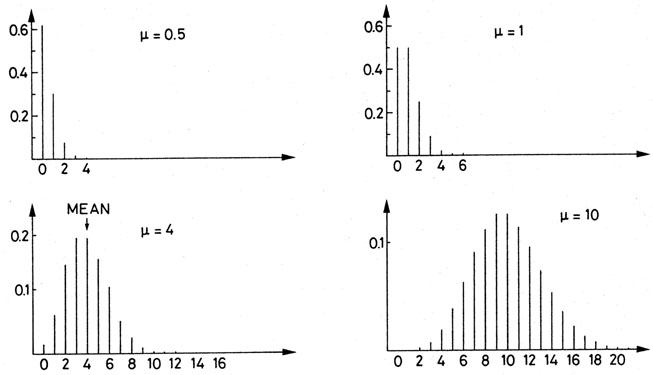
Fig. 2. Poisson distribution for various values of µ.

Figure 2 plots the Poisson distribution for various values of µ. Note that the distribution is not symmetric. The peak or maximum of the distribution does not, therefore, correspond to the mean. However, as µ becomes large, the distribution becomes more and more symmetric and approaches a Gaussian form. For µ 20, a Gaussian distribution with mean µ and variance ² = µ, in fact, becomes a relatively good approximation and can be used in place of the Poisson for numerical calculations. Again, one must neglect the fact that we are replacing a discrete distribution by a continuous one.