 INTRODUCTION
THE COSMIC INVENTORY
GLOBAL ABUNDANCES AND YIELDS
COSMIC STAR FORMATION AND CHEMICAL EVOLUTION: GCE VS
HDF
EXTRAGALACTIC BACKGROUND LIGHT
REFERENCES
To be published in "Vulcano Workshop: Chemical Enrichment of
Intracluster and Intergalactic Medium", May 14 - 18 2001,
eds. F. Matteucci and F. Giovannelli, ASP Conference Series;
astro-ph/0107215
Abstract. An attempt is made to guess the overall cosmic abundance of "metals" and the contribution made by the energy released in their production to the total intensity of extragalactic background light (EBL). With a comparable or somewhat larger amount coming from white dwarfs, and a probably quite modest contribution from AGNs, one can fairly easily account for the lower end of the range of existing estimates for the total EBL intensity (50 to 60 nwt m-2 sterad-1), but it seems more difficult should some higher estimates (90 to 100 in the same units) prove to be correct.
Table of Contents
INTRODUCTION
THE COSMIC INVENTORY
GLOBAL ABUNDANCES AND YIELDS
COSMIC STAR FORMATION AND CHEMICAL EVOLUTION: GCE VS
HDF
EXTRAGALACTIC BACKGROUND LIGHT
REFERENCES
There are certain more or less well or badly determined integral constraints on the past history of star formation in the universe. These include
 B, now fairly
well determined both from primordial deuterium
(O'Meara et al 2001)
and from the CMB fluctuation spectrum (e.g.
Turner 2001).
B, now fairly
well determined both from primordial deuterium
(O'Meara et al 2001)
and from the CMB fluctuation spectrum (e.g.
Turner 2001).
*,
rather less well determined as it
involves a combination of luminosity-density measurements with an IMF
and evolutionary population synthesis models.
Z, due to the
heavy-element content of stars, the interstellar medium and the
intergalactic medium, a quantity that is very poorly known and largely
a matter of guesswork. In this talk I shall nevertheless make some guesses,
so that at least one can see more easily how things relate to one another.
In particular, the metallicity
ZIGM of the intergalactic
medium has tended to be either neglected or underestimated in models of
the past star formation
rate, and it is of interest to ask about its relation with EBL.
A useful starting point is the cosmic baryon budget drawn up by Fukugita, Hogan & Peebles (1998), hereinafter FHP, shown in the accompanying table. The total from Big Bang nucleosynthesis (BBNS) adopted here agrees quite well with the amount of intergalactic gas at a red-shift of 2 to 3 deduced from the Lyman forest, but exceeds the present-day stellar (plus cold gas) density by an order of magnitude. (1)
| All baryons from BBNS | |
| (D/H = 3 × 10⁻⁵ a) | 0.04 h70-2 |
| Stars in spheroids | 0.0026 h70-1 b |
| Stars in disks | 0.0009 h70-1 b |
| Total stars | 0.0035 h70-1 b |
| Cluster hot gas | 0.0026 h70-1.5 b |
| Group/field hot gas | 0.014 h70-1.5 b (0.004h75-1 in O VI systems c) |
| Total stars + gas | 0.021 h70-1.5 b |
| Machos + LSB gals | ?? b |
|
Z (stars,
Z = 0.02 d)
| 7 × 10⁻⁵ h70-1 |
|
Z (hot gas,
Z = .006)
| 1.0 × 10⁻⁴ h70-1.5 b |
| 1.2 × 10⁻⁴ h70-1.3 e | |
Yield
 Z
/ * Z
/ *
| 0.051 h70-0.3
( 3Z
3Z !) !)
|
Damped Ly- (H I)
(H I)
| 0.0015 h70-1 b, f |
| Ly- forest
(H+)
| 0.04 h70-2 b, g |
| Gals + DM halos | |
| (M/L = 210 h70) | 0.25 b, h |
| All matter | |
| (fB = .056 h-1.5) | 0.37 h70-0.5 b, i |
| a O'Meara et al 200l; but see also Pettini & Bowen 2001; b Fukugita, Hogan & Peebles 1998; c Tripp, Savage & Jenkins 2000; d Edmunds & Phillipps 1997; e Mushotzky & Loewenstein 1997; f Storrie-Lombardi, Irwin & MacMahon 1996; g Rauch, Miralda-Escudé, Sargent et al 1998; h Bahcall, Lubin & Dorman 1995; i White & Fabian 1995. | |
FHP pointed out that a dominant and uncertain contribution to the
baryon budget comes from intergalactic ionized gas, not readily
detectable because of its high temperature and low density. The number
which I quote is based on the assumption that the spheroid
star-to-gravitational mass ratio and baryon fraction are the same in
clusters and the field, an assumption that had also been used previously by
Mushotzky & Loewenstein
(1997).
The resulting total star-plus-gas density
is within spitting distance of
B from BBNS, but
leaves a
significant-looking shortfall which may be made up by some combination
of MACHOs and low surface-brightness galaxies; it is not clear that a
significant contribution from the latter has been ruled out (cf
O'Neil 2000).
1 The stellar density taken here from
FHP is based on B-luminosity density estimates and might be revised
upwards by 50 per cent in light of SDSS commissioning data
(Blanton et al 2000)
or downwards by 20 per cent in light of 2dF red-shifts plus
2MASS K-magnitudes
(Cole et al 2000);
in either case we are following FHP in assuming the IMF by
Gould, Bahcall & Flynn
(1996),
which has 0.7 times the
M / LV ratio for old stellar populations
compared to a Salpeter function with lower cutoff at
0.15 M.
Back.
We now have the tricky task of estimating the total heavy-element content
of the universe. Considering stars alone, it seems reasonable to adopt
solar Z as an average, but the total may be dominated by the
still unseen
intergalactic gas, which Mushotzky & Loewenstein argue to have the same
composition as the hotter, denser gas seen in clusters of galaxies, i.e.
about 1/3 solar. (2)
It could be the case, though, that the metallicity
of the IGM is substantially lower in light of the metallicity-density
relation predicted by
Cen & Ostriker (1999)
and in that of the low metallicities found in low red-shift
Ly- clouds by
Shull et al (1998).
Against this, we have
neglected any metals contained in LSB galaxies or whatever makes up the
shortfall between
IGM and
B, so we are being
conservative in our estimate of
Z.
The mass of heavy elements in the universe is related to that of stars
through the yield, defined as the mass of "metals" synthesised and
ejected by a generation of stars divided by the mass left in form of
long-lived stars or compact remnants
(Searle & Sargent
1972).
The yield may be predicted by a combination of an IMF with models of
stellar
yields as a function of mass, or deduced empirically by applying a
galactic chemical evolution (GCE) model to a particular region like the
solar neighbourhood and comparing with abundance data. E.g.
Fig 1 shows
an abundance distribution function for the solar neighbourhood plotted in
a form where in generic GCE models the maximum of the curve gives the
yield directly, and it is a bit below
Z. Similar
values are predicted theoretically using fairly steep IMFs like that of
Scalo (1986).
In Table 1, on the other hand, if we
divide the mass of metals
by the mass of stars, we get a substantially higher value, corresponding
to a more top-heavy IMF.

|
Figure 1. Oxygen abundance distribution function in the solar neighbourhood, after Pagel & Tautvaisiene (1995). |
There are two other indications for a top-heavy IMF, one local and one
in clusters of galaxies themselves. The local one is an investigation by
Scalo (1998)
of open clusters in the Milky Way and the LMC, where he plots
the IMF slopes found as a function of stellar mass. The scatter is large,
but on average he finds a Salpeter slope above
0.7M and a
virtually flat relation (in the sense
dN / dlogm
0) below,
which could quite easily account for the sort of yield found in
Table 1.
The other indication is just the converse of the argument we have already
used in guessing the abundance in the IGM: the mass of iron in the
intra-cluster gas is found
(Arnaud et al 1992)
to be
| (1) |
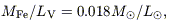
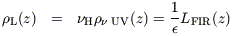
where LV is the luminosity of E and S0 galaxies in the cluster. As has been pointed out by Renzini et al (1993) and Pagel (1997), given a mass:light ratio less than 10, we then have

| (2) |
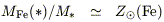
| (3) |

| (4) |
The argument is very simple; the issue is just whether such high yields are universal or confined to elliptical galaxies in clusters.
2 This refers to iron abundance, the relation of which to the more energetically relevant quantity Z is open to some doubt. Papers given at this conference indicate an SNIa-type mixture in the immediate surroundings of cD galaxies with maybe a more SNII-like mixture in the intra-cluster medium in general; for simplicity I assume the mixture to be solar. Back.
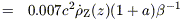
The deduction of past star formation rates from rest-frame UV radiation in the Hubble and other deep fields as a function of red-shift is tied to "metal" production through the Lilly-Cowie theorem (Lilly & Cowie 1987):
| (5) |
| (6) |

| (7) |
where (1 + a) 2.6 is
a correction factor to allow for production
of helium as well as conventional metals and
 (probably between
about 1/2 and 1) allows for nucleosynthesis products falling back into
black-hole remnants from the higher-mass stars.
(probably between
about 1/2 and 1) allows for nucleosynthesis products falling back into
black-hole remnants from the higher-mass stars.
 is the fraction
of total energy output absorbed and re-radiated by dust and
is the fraction
of total energy output absorbed and re-radiated by dust and
 H
is the frequency at the Lyman limit (assuming a flat spectrum at lower
frequencies). The advantage of this formulation is that the relationship
is fairly insensitive to details of the IMF.
H
is the frequency at the Lyman limit (assuming a flat spectrum at lower
frequencies). The advantage of this formulation is that the relationship
is fairly insensitive to details of the IMF.
Eq (7) is the same as eq (13) of
Madau et al (1996),
so I refer to the metal-growth rate derived in this way as
 Z(conventional).
Assuming a Salpeter IMF from 0.1 to
100 M with
all stars above 10
M expelling
their synthetic products in SN explosions,
one then derives a conventional SFR density through multiplication with
the magic number 42:

| (8) |
In general, we shall have
| (9) |
where  is some
factor. E.g., for the IMF adopted by FHP,
= 0.67, whereas for the
Kroupa-Scalo one
(Kroupa et al 1993)
= 2.5.
is some
factor. E.g., for the IMF adopted by FHP,
= 0.67, whereas for the
Kroupa-Scalo one
(Kroupa et al 1993)
= 2.5.
Finally, the present stellar density is derived by integrating over the past SFR and allowing for stellar mass loss in the meantime, and the metal density is related to this through the yield, p:
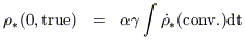
| (10) |
| (11) |
(where is the lockup
fraction), whence (if a = 1.6)

| (12) |
which can be compared with
Z
1/60. It was pointed out by
Madau et al (1996)
that the Salpeter slope gives a better fit to the
present-day stellar density than one gets from the steeper one - a
result that is virtually independent of the low-mass cutoff if one
assumes a power-law IMF.
Eq (8), duly corrected for absorption, forms the basis for numerous
discussions
of the cosmic past star-formation rate or "Madau plot". Among the more
plausible ones are those given by
Pettini (1999)
shown in Fig 2 and by
Rowan-Robinson (2000),
which leads to similar results and is shown to
explain the far IR data. Taking
= 0.62 (corresponding to a
Salpeter IMF that is flat below
0.7M) rather
than Pettini's value of 0.4 (for an IMF truncated at
1M), and
= 0.7, we get the
data in the following table.
|
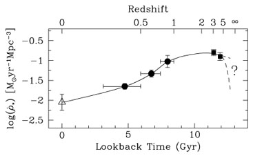
Figure 2. Global comoving star formation rate density vs. lookback time compiled from wide-angle ground-based surveys (Steidel et al. 1999 and references therein) assuming E-de S cosmology with h = 0.5, after Pettini (1999). Courtesy Max Pettini. |
Table 2 indicates that the known stars are
roughly accounted for by the
history shown in Fig 2 (or by Rowan-Robinson)
and the metals also if
is close to unity, i.e. the
full range of stellar masses expel
their nucleosynthesis products. At the very least,
has to be 1/2,
to account for metals in stars alone. The other point arising from the
table, made by Pettini, is that at a red-shift of 2.5, 1/4 of the stars
and metals have already been formed, but we do not know where the
resulting metals reside.
| z = 0 | z = 2.5 | |
*
=
 *(conv.) dt
| 3.6 × 10⁸
M
Mpc-3
| 9 × 10⁷
M
Mpc-3
|
|
*
= * /
1.54 × 10¹¹ h702
| .0024h70-2 | 6 × 10⁻⁴ h70-2 |
|
*(FHP 98)
| .0035h70-1 | |
|
Z
= p
*
= * /
(42
)
| 2.0 × 10⁷
M
Mpc-3
| 5 × 10⁶
M
Mpc-3
|
|
Z (predicted)
| 1.3 × 10⁻⁴
h70-2
| 3.2 × 10⁻⁵
h70-2
|
|
Z (stars,
Z = Z)
| 7 × 10⁻⁵ h70-1 | |
|
Z (hot gas,
Z =
0.3Z)
| 1.0 × 10⁻⁴h70-1.5 | |
-> 0.5  1.3
1.3
| ||
|
Z (DLA,
Z =
0.07Z)
| 2 × 10⁻⁶ h70-1 | |
|
Z (Ly. forest,
Z =
0.003Z)
| 1 × 10⁻⁶ h70-2 | |
|
Z (Ly. break gals,
Z =
0.3Z)
| ? | |
|
Z (hot gas)
| ? | |

|
Figure 3. Spectrum of extragalactic
background light, based on COBE data after
Hauser 2001
(diamonds with error bars, dotted and short-dash curves),
Madau & Pozzetti 2000
(squares),
Totani et al 2001
(crosses),
Bernstein, Freedman &
Madore 2001
(triangles) and
Armand et al 1994
(asterisk). The broken-line curve
(Biller et al 1998)
and horizontal dash-dot line
(Hauser 2001)
show upper limits based on lack of attenuation of high-energy
|
Fig 3 shows the spectrum of extragalactic
background light (EBL) with the model fit by
Pei, Fall & Hauser
(1999).
Gispert, Lagache & Puget
(2000)
have estimated the total EBL
I
d based on observation to lie
within the following limits:
 6µm:
6µm:
| 20 to 40 | nwt | m-2 | sterad-1 |
|
> 6µm:
| 40 to 50 | " | " | " |
| Total: | 60 to 90 | " | " | " |
(The total from the model of Pei, Fall & Hauser (1999) is 55 in these units.)
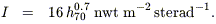
We use the estimates of stellar and metal densities in Tables 1 and 2 together with eq (7) and an assumption about the mean red-shift of metal formation to derive the EBL contributions from:
= 0.02:

| (13) |
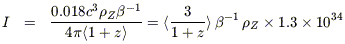
| (14) |

| (15) |
0.007:

| (16) |
| (17) |
Here we use eq (6) without the (1 + a), since most of the nuclear energy is already released on reaching this stage. Assuming most stars to belong to an old population so that

| (18) |
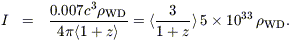
| (19) |
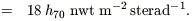
| (20) |
Madau & Pozzetti (2000) and Brusa, Comastri & Vignali (2001) have made estimates of the AGN contribution to EBL based on the the abundance of massive black holes and that of obscured hard X-ray sources, respectively. They agree that the contribution is quite small, of order 5 nwt m-2 sterad-1.
The upshot is that these readily identifiable contributions add up to 48 nwt m-2 sterad-1, well within range (given the obvious uncertainties in mean z and other parameters) of the lower estimate given at the beginning of this section. It is interesting to note that white dwarfs and intergalactic metals come out as the major contributors, either one predominating over metallicity in known stars. To reach the higher estimate may involve some more stretching of the parameters.
I thank Richard Bower, Jon Loveday and Max Pettini for helpful information and comments.