


For 4 He, we follow an analogous procedure to that described
above. We again start with a set of observed quantities: line intensities
I( ) which include
the reddening correction previously
determined and its associated uncertainty which also includes the
uncertainty in
C(H
) which include
the reddening correction previously
determined and its associated uncertainty which also includes the
uncertainty in
C(H ); the
equivalent width
W(); and
temperature t. The Helium line intensities are scaled to
H
and the singly ionized helium abundance is given by
); the
equivalent width
W(); and
temperature t. The Helium line intensities are scaled to
H
and the singly ionized helium abundance is given by
| (C1) |
where E() /
E(H) is the
theoretical emissivity scaled
to H. The expression
(C1), also contains a correction
factor for underlying stellar absorption, parameterized now by
aHeI,
a density dependent collisional correction factor,
(1 +  )-1, and a
florescence correction which
depends on the optical depth
)-1, and a
florescence correction which
depends on the optical depth  .
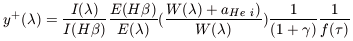
Thus y+ implicitly
depends on three unknowns, the electron density, n,
aHeI, and .
.
Thus y+ implicitly
depends on three unknowns, the electron density, n,
aHeI, and .
To be definite, we list here the necessary components in expression
(C1). The theoretical emissivities scaled
to H are taken from
Smits (1996):
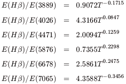
| (C2) |
Our expressions for the collisional correction
, are taken from
Kingdon & Ferland
(1995).
We list them here for completeness. They are:
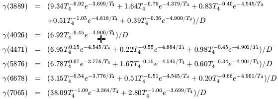
| (C3) |
where D = 1 + 3130n-1
T4-0.50.
The corrections for florescence are given in terms of the optical depth
for the He I 3389 line. We use the IT98 fit
of the
Robbins (1968)
enhancement factors:
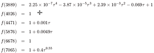
| (C4) |
f (4026) is not given by IT98, but is assumed to be 1 because it is a
singlet line (as is the case for
6678).
Once the individual values for
y+() are
determined, we can
begin the process for self-consistently determining the physical
parameters. As described in the text, we may wish to consider 3, 5, or 6
different 4 He emission lines. Depending on the number of
lines used, we next determine the average helium abundance.

| (C5) |
This is a weighted average, where the uncertainty
 () is found by propagating the
uncertainties in the
observational quantities stemming from the observed line fluxes (which
already contains the uncertainty due to
C(H), the equivalent
widths, and input temperature. Since the average,
, depends on
the parameters, n, and
aHeI, we must make an initial estimate for these.
() is found by propagating the
uncertainties in the
observational quantities stemming from the observed line fluxes (which
already contains the uncertainty due to
C(H), the equivalent
widths, and input temperature. Since the average,
, depends on
the parameters, n, and
aHeI, we must make an initial estimate for these.
From , we can
define a
 2 as the deviation of the
individual He abundances
y+()
from the average,
2 as the deviation of the
individual He abundances
y+()
from the average,
| (C6) |
We then minimize 2,
to determine n, aHeI, and
.
Uncertainties in the output parameters are determined as in the
case for aHI and
C(H), that is by
varying the outputs until  2 = 1. Propagation in the
latter uncertainties give us a
reasonable handle on the systematic uncertainties in our final result for
y+.
2 = 1. Propagation in the
latter uncertainties give us a
reasonable handle on the systematic uncertainties in our final result for
y+.
This procedure differs somewhat from that proposed by IT98, in that the
2 above (C6) is a
straight weighted average, whereas IT98
minimize the differences between ratios of He abundances from pairs of
He I lines (referenced to one wavelength,
typically 4471). When the reference line is particularly sensitive to a
systematic effect such as underlying stellar absorption, the uncertainty
propagates to all lines this way. In our case, the individual
uncertainties in the line strengths are kept separate.
Finally, as in the case for the hydrogen lines, we have performed a
Monte-Carlo simulation of the data to test the robustness of the
solution for n, aHeI, and
from the
2 minimization and
the true uncertainty in these quantities.
As before, starting with the observational inputs and their stated
uncertainties, we have generated a data set which is Gaussian
distributed for the 6 observed He
emission lines (plus the temperature). From each distribution, we
randomly select a set of input values and run the
2 minimization. The
selection of data is repeated 1000 times. We
thus obtain a distribution of solutions for
n, aHeI, and
,
and we compare the mean and dispersion of these distributions with the
initial solution for these quantities.