Cosmological Dynamics - E. Bertschinger

2. Eulerian fluid dynamics

A fluid is a dense set of particles treated as a continuum. If particle collisions are rapid enough to establish a local thermal equilibrium (e.g., Maxwell-Boltzmann velocity distribution), the fluid is an ideal collisional gas. If collisions do not occur (e.g., a gas of dark matter particles), the gas is called collisionless. (I exclude incompressible fluids, i.e., liquids, from consideration because the gases considered in cosmology are generally very dilute and compressible.) The fluid equations discussed in this lecture apply only for a collisional gas (or a pressureless collisionless gas). They apply, for example, to baryons (hydrogen and helium gas) after recombination, to cold dark matter before trajectories intersect ("cold dust"), and (with relativistic corrections) to the coupled photon-baryon fluid before recombination.

I shall assume a nonrelativistic gas and ignore bulk electric and magnetic forces. These are not difficult to add, but the essential physics of cosmological fluid dynamics does not require them.

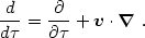
The fluid equations consist of mass and momentum conservation laws and an equation of state. Mass conservation is represented by the continuity equation. In proper coordinates (r, t) this is

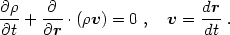(2.1)

We convert to comoving coordinates tau = integ dt / a(t), x = r / a(t), being careful to transform the partial derivatives as follows: partial / partial t = ( partial tau / partial t) partial / partial tau + ( partial x / partial t) ^. partial / partial x, partial / partial r = a^-1 partial / partial x ident a^-1 nabla . We also rewrite the density and velocity by factoring out the mean behavior:

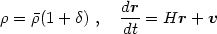(2.2)

where v = dx / d tau is now the peculiar velocity. The reader may easily show that eq. (2.1) becomes

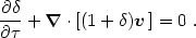(2.3)

Momentum conservation for an ideal fluid is represented by the Euler equation (Landau & Lifshitz 1959). It is most simply obtained by adding the pressure-gradient force to the equation of motion for a freely-falling mass element, eq. (1.7). In comoving coordinates, we find

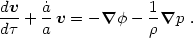(2.4)

The time derivative is taken along the fluid streamline and is known as the convective or Lagrangian time derivative:

(2.5)

Closing the fluid equations requires an evolution equation for the pressure or some other thermodynamic variable. Perhaps the most natural is the entropy. For a collisional gas, thermodynamics implies an equation of state p = p( rho , S) where S is the specific entropy. For example, for an ideal nonrelativistic monatomic gas, for reversible changes we have

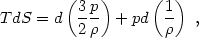(2.6)

which says that the heat input to a fluid element equals the change in thermal energy plus the pressure work done by the element, i.e., energy is conserved. Combining this with the ideal gas law p = rho k_BT / µ where µ is the mean molecular mass and k_B is the Boltzmann constant, we obtain

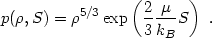(2.7)

The equation of state must be supplemented by an evolution equation for the specific entropy. Outside of shock waves, the entropy evolution equation is

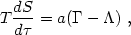(2.8)

where Gamma and Lambda are, respectively, the proper specific heating and cooling rates (in erg g^-1 s^-1). They are determined by microphysical processes such as radiative emission and absorption, cosmic ray heating, Compton processes, etc. For the simplest case, adiabatic evolution, Gamma = Lambda = 0. For a realistic non-ideal gas, it may be necessary to evolve the radiation field, the ionization fraction, and other variables specifying the equation of state.

The fluid equations are much harder to solve than Newton's laws for particles falling under gravity, for several reasons. First, they are nonlinear partial differential equations rather than a set of coupled ordinary differential equations. Second, shock waves (discontinuities in rho , p, S, and v) prevent intersection of fluid elements. These discontinuities must be resolved (on a computational mesh or otherwise) and followed stably and accurately. Finally, heating and cooling for realistic gases are complicated and can lead to large temperature or entropy gradients that are difficult to resolve. An example of the latter is the sun, whose temperature changes by about 15 million K in a distance that is minuscule compared with cosmological distance scales.

Computational fluid dynamics is a difficult art but is important for galaxy formation. I shall not summarize the numerical methods here but refer the reader instead to the literature (e.g., Sod 1985, Leveque 1992, Monaghan 1992, Bryan et al. 1994, Kang et al. 1994).

Some of the most important effects of gas pressure can be gleaned from linear perturbation theory, in which we linearize the fluid equations about the uniform solution for an unperturbed Robertson-Walker spacetime. This technique is useful for checking for gravitational and other linear instabilities. Moreover, the linearized fluid equations may provide a reasonable description of large-scale, small-amplitude fluctuations in the (dark+luminous) matter, even if structure is nonlinear on small scales. This is a common assumption in large-scale structure theory. It is supported reasonably well by numerical simulations.

Linearizing the continuity and Euler equations gives

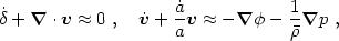(2.9)

where an overdot denotes partial / partial tau . The pressure gradient may be obtained from the equation of state p = p( rho , S). For an ideal nonrelativistic monatomic gas,

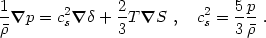(2.10)

Finally, we must linearize the entropy evolution equation. If the time scale for entropy changes is long compared with the acoustic or gravitational time scales, eq. (2.8) becomes dS / d tau approx 0. For the small peculiar velocities of linear perturbation theory this reduces to S dot approx 0.

There are five fluid variables ( rho , S, and three components of v), hence five linearly independent modes. The general linear perturbation is a linear combination of these, which we now proceed to examine.