4.5. Gauge modes

As we noted above, the synchronous gauge conditions do not completely fix the spacetime coordinates because of the freedom to redefine the perturbed constant-time hypersurfaces and to reassign the spatial coordinates within these hypersurfaces. This freedom is not obvious in the linearized Einstein equations for the scalar and vector modes, but it is present in the form of additional solutions that must be fixed by appropriate choice of initial conditions and that represent nothing more than relabeling of the coordinates in an unperturbed Robertson-Walker spacetime.

To see this effect more clearly, we consider a general infinitesimal coordinate transformation from (, xⁱ) to (, ⁱ), known as a gauge transformation:

(4.39)

For convenience we have split the spatial transformation into longitudinal and transverse parts. Note that the transformed time and space coordinates depend in general on all four of the old coordinates.

Coordinate freedom leads to ambiguity in the meaning of density perturbations. Consider, for example, the simple case of an unperturbed Robertson-Walker universe in which the density depends only on (if one uses the "correct" coordinate). In the transformed system it depends also on ⁱ: () = () + ( )(x, ). In other words, even in an unperturbed universe we can be fooled into thinking there are spatially-varying density perturbations.

This example may seem contrived, but the ambiguity is not trivial to avoid: When spacetime itself is perturbed, and time is not absolute, what is the best choice of time? The same question arises for the spatial coordinates.

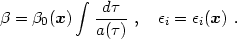
To clarify this situation we must examine gauge transformations further. First note that when we transform the coordinates we must also transform the metric perturbation variables so that the line element ds² (a spacetime scalar) is invariant. It is straightforward to do this using eqs. (4.11) and (4.39). The result is

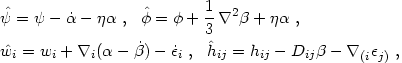(4.40)

where D_ij is the traceless double gradient operator defined in eq. (4.15). The transformed fields (with carets) are to be evaluated at the same coordinate values (, xⁱ) as the original fields.

Suppose now that our original coordinates satisfy the synchronous gauge conditions = w_i = 0. [To recover the notation of eq. (4.27) used specially for synchronous gauge we now double h_ij and put the trace of h_ij into h = - 6.] From eqs. (4.40) and (4.27) it follows that there is a whole family of synchronous gauges with metric variables related to the original ones by

(4.41)

where

(4.42)

Thus, the synchronous gauge has residual freedom in the form of one scalar (₀) and one transverse vector (_i) function of the spatial coordinates.

The presence of these extraneous solutions (called gauge modes) has created a great deal of confusion in the past, which might have been avoided had more cosmologists read the paper of Lifshitz (1946). In 1980, Bardeen wrote an influential paper showing how one may take linear combinations of the metric and matter perturbation variables that are free of gauge modes. For example, Bardeen defined two scalar perturbations _A and _H related to our synchronous gauge variables h and (Bardeen actually used the variables H_L h/6 and H_T - /2) as follows:

(4.43)

It is easy to check that these variables are invariant under the synchronous gauge transformation given by eqs. (4.41)-(4.42).

Bardeen's work led to a flurry of papers concerning gauge-invariant variables in cosmology. A standard reference is the classic paper by Kodama & Sasaki (1984). Elegant treatments based on general 3+1 splitting of spacetime were given later by Durrer & Straumann (1988) and Bardeen (1989). The simpler form of the gauge-invariant variables often makes it easier to find analytical solutions (e.g., Rebhan 1992). However, it is not necessary to use gauge-invariant variables during a calculation, and many cosmologists have continued successfully to use synchronous gauge. In the end, when the results are converted to measurable quantities - spacetime scalars - the gauge modes automatically get canceled. In a numerical solution, however, one must be careful that the gauge modes do not swamp the physical ones, otherwise roundoff can produce significant numerical errors.

Gauge invariant variables actually appear somewhat strange if we consider the analogous situation in electromagnetism. The electric and magnetic fields in flat spacetime may be obtained from potentials and A (note we are implicitly using a 3+1 split of spacetime),

(4.44)

With this choice, the source-free Maxwell equations are automatically satisfied; the other two (the Coulomb and Ampère laws) become

(4.45)

where is the charge density and J is the current density. These equations are invariant under the gauge transformation = - , = A_i + _i .

If we didn't know about electric and magnetic fields, but were alarmed by the gauge-dependence of the potentials, we could try to find linear combinations of and A that are gauge-invariant. However, there are two well-known and more direct ways to eliminate gauge modes. The first is "gauge fixing" - i.e., placing constraints on the potentials so as to eliminate gauge degrees of freedom. One popular choice, for example, is the Coulomb gauge ^. A = 0, so that A = A is transverse. The transversality condition means that the gauge transformation variable cannot depend on position (though it can depend on time); thus, most of the gauge freedom is eliminated. The second possibility is to work with the physical fields themselves instead of the potentials: E and B are automatically gauge-invariant. This procedure requires that we analyze the equation of motion for charges to determine which combinations of and A are physically most significant.

In the next section we shall adopt the first procedure (gauge-fixing) using the gravitational analogue of the Coulomb gauge. Later we shall introduce Ellis' covariant approach based on gravitational fields themselves.