3.5. The dual formalism

The usual procedure for treating a specific cosmic string dynamical problem consists in writing and varying an action which is assumed to be the integral over the worldsheet of a Lagrangian function depending on the internal degrees of freedom of the worldsheet. In particular, for the structureless string, this is taken to be the Goto-Nambu action, i.e. the integral over the surface of the constant string tension. In more general cases, various functions have been suggested that supposedly apply to various microscopic field configurations. They share the feature that the description is achieved by means of a scalar function , identified with the phase of a physical field trapped on the string, whose squared gradient, namely the state parameter w, has values which completely determine the dynamics through a Lagrangian function (w). This description has the pleasant feature that it is easily understandable, given the clear physical meaning of . However, as we shall see, there are instances for which it is not so easily implemented and for which an alternative, equally valid, dual formalism is better adapted [Carter, 1989].

Macroscopic equation of state

But first, let us concentrate on the macroscopic equation of state. At this point, it is clear that conducting strings have a considerably richer structure than Goto-Nambu strings. In particular, Witten strings have and internal structure with its own equation of state U = U(T). This, in turn, allows us to compute the characteristic perturbations speeds [Carter, 1989] :

• A transverse (wiggle) speed c²_T = T / U for extrinsic perturbations of the worldsheet.
• A longitudinal (`woggle') speed c²_L = -dT / dU for sound-type perturbations within the worldsheet.

Of course, these characteristic speeds are not defined for a structureless Goto-Nambu string, but are fully meaningful for any other model. Numerical results for Witten strings by Peter [1992] yield c_L < c_T, i.e. the regime is supersonic.

We will now explore the different ansätze proposed in the literature over the years. Clearly, the simplest case is that one without any currents, namely the Goto-Nambu action. In the present formalism it is expressed by the action

(43)

which is proportional to string worldsheet area. The corresponding Lagrangian is given simply by _GN = -m² and its equation of state results U = T = m².

The first thing that comes to the mind when trying to extend this simple action to the case including currents is of course to add a small (linear) term proportional to the state parameter w, which itself includes the relevant information on the currents. Hence, a first try would be _linear = -m² - w / 2. It turns out that this simple model is also self-dual (with _linear = -m² - / 2], to be precised below) and the equation of state resulting is (for both electric and magnetic regimes) U + T = 2m². However, it follows that c_T < c_L = 1, i.e., the model is subsonic and this goes at odds with the numerical results for Witten strings.

2nd try: keeping with minimal modifications autour the Goto-Nambu solution, another, Kaluza-Klein inspired, model was proposed: _KK = -m[m² + w]^1/2. This model is also self-dual and the resulting equation of state is UT = m⁴. Moreover, in the limit of small currents it reproduces the linear model of the last paragraph. However, this time both characteristic perturbation speeds are equal and smaller than unity, c_T = c_L < 1, i.e. the model is transonic and this fact disqualifies it for modeling Witten strings.

At this point, one may think that there is an additional relevant parameter in the theory, the scale associated with the current-carrier mass, which we shall note m_* (= m). It is only by introducing this extra mass scale that the precise numerical solutions for Witten strings can be recovered. Two models were proposed, the first one with

(44)

for which we get the amplitude of the -condensate ^-1 = (1 + (w / m²_*))^-2 (recall that it was ^-1 dx dy ||² and C |w|^1/2 dx dy ||²). This ansatz fits well the w -m² divergence in the macroscopic charge density C [see Figure (1.8)] and it is the best choice for spacelike currents.

The second model is given by

(45)

and we get ^-1 = (1 + w / m²_*)^-1. This one is the best for timelike currents and is OK for spacelike currents as well [Carter & Peter, 1995].

These two two-scale models we will employ below to study the dynamics of conducting string loops and the influence of electromagnetic self-corrections on this dynamics at first order between the current and the self-generated electromagnetic field. But before that, let us introduce the formal framework we need for the job.

The dual formalism

Here we will derive in parallel expressions for the currents and state parameters in two representations, which are dual to each other. This will not be specific to superconducting vacuum vortex defects, but is generally valid to the wider category of elastic string models [Carter, 1989]. In this formalism one works with a two-dimensional worldsheet supported master function () considered as the dual of (w), these functions depending respectively on the squared magnitude of the gauge covariant derivative of the scalar potentials and as given by

(46)

where ₀ and ₀ are adjustable, respectively positive and negative, dimensionless normalization constants that, as we will see below, are related to each other. The arrow in the previous equation stands to mean an exact correspondence between quantities appropriate to each dual representation.

In Eq. (46) the scalar potentials and are such that their gradients are orthogonal to each other, namely

(47)

implying that if one of the gradients, say _|a is timelike, then the other one, say _|a, will be spacelike, which explains the different signs of the dimensionless constants ₀ and ₀.

Whether or not background electromagnetic and gravitational fields are present, the dynamics of the system can be described in the two equivalent dual representations which are governed by the master function and the Lagrangian scalar , that are functions only of the state parameters and w, respectively. The corresponding conserved current vectors, n^a and z^a, in the worldsheet, will be given according to the Noetherian prescription

(48)

This implies

(49)

where we use the induced metric for internal index raising, and where and can be written as

(50)

As it will turn out, the equivalence of the two mutually dual descriptions is ensured provided the relation

(51)

holds. This means one can define in two alternative ways, depending on whether it is seen it as a function of or of . We shall therefore no longer use the function in what follows.

Based on Eq. (47) that expresses the orthogonality of the scalar potentials we can conveniently write the relation between and as follows

(52)

where is the antisymmetric surface measure tensor (whose square is the induced metric, _ab ^b_c = _ac). From this and using Eq. (46) we easily get the relation between the state variables,

(53)

Both the master function and the Lagrangian are related by a Legendre type transformation that gives

(54)

The functions and can be seen [Carter, 1997] to provide values for the energy per unit length U and the tension T of the string depending on the signs of the state parameters and w. (Originally, analytic forms for these functions and were derived as best fits to the eigenvalues of the stress-energy tensor in microscopic field theories). The necessary identifications are summarized in Table 1.2.

Table 1.2. Values of the energy per unit length U and tension T depending on the timelike or spacelike character of the current, expressed as the negative values of either or .

Equations of state for both regimes
regime	U	T	and w	current
electric	-	-	< 0	timelike
magnetic	-	-	> 0	spacelike

This way of identifying the energy per unit length and tension with the Lagrangian and master functions also provides the constraints on the validity of these descriptions: the range of variation of either w or follows from the requirement of local stability, which is equivalent to the demand that the squared speeds c_E² = T / U and c_L² = -dT / dU of extrinsic and longitudinal (sound type) perturbations be positive. This is thus characterized by the unique relation

(55)

which should be equally valid in both the electric and magnetic ranges. Having defined the internal quantities, we now turn to the actual dynamics of the worldsheet and prove explicitly the equivalence between the two descriptions.

Equivalence between and

The dynamical equations for the string model can be obtained either from the master function or from the Lagrangian in the usual way, by applying the variation principle to the surface action integrals

(56)

and

(57)

(where det{_ab}) in which the independent variables are either the scalar potential or the phase field on the worldsheet and the position of the worldsheet itself, as specified by the functions x^µ{, }.

Independently of the detailed form of the complete system, one knows in advance, as a consequence of the local or global U(1) phase invariance group, that the corresponding Noether currents will be conserved, namely

(58)

For a closed string loop, this implies (by Green's theorem) the conservation of the corresponding flux integrals

(59)

meaning that for any circuit round the loop one will obtain the same value for the integer numbers N and Z, respectively. Z is interpretable as the integral value of the number of carrier particles in the loop, so that in the charge coupled case, the total electric charge of the loop will be Q = Ze. Moreover, the angular momentum of the closed loop turns out to be simply J = Z N.

The loop is also characterized by a second independent integer number N whose conservation is trivially obvious. Thus we have the topologically conserved numbers defined by

(60)

where it is clear that N, being related to the phase of a physical microscopic field, has the meaning of what is usually referred to as the winding number of the string loop. The last equalities in Eqs. (60) follow just from explicitly writing the covariant derivative _|a and noting that the circulation integral multiplying A_µ vanishes. Note however that, although Z and N have a clearly defined meaning in terms of underlying microscopic quantities, because of Eqs. (59) and (60), the roles of the dynamically and topologically conserved integer numbers are interchanged depending on whether we derive our equations from or from its dual .

As usual, the stress momentum energy density distributions ^µ and ^µ on the background spacetime are derivable from the action by varying the actions with respect to the background metric, according to the specifications

(61)

and

(62)

This leads to expressions of the standard form, i.e. expressible as an integral over the string itself

(63)

in which the surface stress energy momentum tensors on the worldsheet (from which the surface energy density U and the string tension T are obtainable as the negatives of its eigenvalues) can be seen to be given by

(64)

where the (first) fundamental tensor of the worldsheet is given by

(65)

and the corresponding rescaled currents ^µ and c^µ are obtained by setting

(66)

Plugging Eqs. (66) into Eqs. (64), and using Eqs. (51), (53) and (54), we find that the two stress-energy tensors coincide:

(67)

This is indeed what we were looking for since the dynamical equations for the case at hand, namely

(68)

which hold for the uncoupled case, are then strictly equivalent whether we start with the action S or with S.

Inclusion of Electromagnetic Corrections

Implementing electromagnetic corrections [Carter, 1997b], even at the first order, is not an easy task as can already be seen by the much simpler case of a charged particle for which a mass renormalization is required even before going on calculating anything in effect related to electromagnetic field. The same applies in the current-carrying string case, and the required renormalization now concerns the master function . However, provided this renormalization is adequately performed, inclusion of electromagnetic corrections, at first order in the coupling between the current and the self-generated electromagnetic field, then becomes a very simple matter of shifting the equation of state, everything else being left unchanged. Let us see how this works explicitly.

Defining K_{µ µ} the second fundamental tensor of the worldsheet, the equations of motion of a charge coupled string read

(69)

where ^µ is the tensor of orthogonal projection to the worldsheet (_µ = g_µ - _µ), F_µ = 2_[µ A_] is the external electromagnetic tensor and j^µ stands for the electromagnetic current flowing along the string, namely in our case

(70)

with r the effective charge of the current carrier in unit of the electron charge e (working here in units where e² 1/137).

Before going on, let us explain a bit the last equations. The above Eq. (69) is no other than an extrinsic equation of motion that governs the evolution of the string worldsheet in the presence of an external field. In fact we readily recognize the external force density acting on the worldsheet f = F_µ j^µ, just a Lorentz-type force with j^µ the corresponding surface current.

Let us also give a simple example where the above seemingly complicated equation of motion proves to be something very well known to all of us. In fact, the above is the two-dimensional analogue of Newton's second law. For a point particle of mass m the Lagrangian is = -m, which implies that its stress energy momentum tensor is given by ^µ = m u^µ u (with u^µ u_µ = -1, for the unit tangent vector u^µ of the particle's worldline). Then, the first fundamental tensor is ^µ = - u^µ u. From this it follows that the second fundamental tensor can be constructed, giving K_µ = u_µ u . Hence, the extrinsic equation of motion yields m = _µ f^µ, i.e., the external to the worldline force _µ f^µ being equal to the mass times the acceleration [Carter, 1997b].

As we mentioned, we are now interested in Eq. (69) which is the natural generalization to two dimensions of Newton's second law. But now we want to include self interactions. The self interaction electromagnetic field on the worldsheet itself can be evaluated [Witten, 1985] and one finds

(71)

with

(72)

where is an infrared cutoff scale to compensate for the asymptotically logarithmic behavior of the electromagnetic potential and m the ultraviolet cutoff corresponding to the effectively finite thickness of the charge condensate, i.e., the Compton wavelength of the current-carrier m^-1. In the practical situation of a closed loop, should at most be taken as the total length of the loop.

The contribution of the self field of Eq. (71) in the equations of motion (69) was calculated by Carter [1997b] and the result is interpretable as a renormalization of the stress energy tensor. That is, the result including electromagnetic corrections is recovered if, in Eq. (61), one uses

(73)

instead of . So, electromagnetic corrections are simply taken into account in the dual formalism employing the master function () unlike the case if we used (w). In fact, it is not always possible to invert the above relation to get an appropriate replacement for the Lagrangian. That the correction enters through a simple modification of () and not of (w) is understandable if one remembers that is the amplitude of the current, so that a perturbation in the electromagnetic field acts on the current linearly, so that an expansion in the electromagnetic field and current yields, to first order in q, + 1/2 j_µ A^µ, which transforms easily into Eq. (73).

One example of the implementation of the above formalism is the study of circular conducting cosmic string loops [Carter, Peter & Gangui, 1997]. In fact, the mechanics of strings developed above allows a complete study of the conditions under which loops endowed with angular momentum will present an effective centrifugal potential barrier. Under certain conditions, this barrier will prevent the loop collapse and, if saturation is avoided, one would expect that loops will eventually radiate away their excess energy and settle down into a vorton type equilibrium state.

If this were the whole story then we would of course be in a big problem, for these vortons, as stable objects, would not decay and would most probably be too abundant to be compatible with the standard cosmology. It may however be possible that in realistic models of particle physics the currents could not survive subsequent phase transitions so that vortons could dissipate. Another way of getting rid of (at least some of) the excess of abundance of these objects is to take account of the electromagnetic self interactions in the macroscopic state of the conducting string: as we said above, the electromagnetic field in the vicinity of the string will interact with the very same string current that generated it, with the resulting effect of modifying its macroscopic equation of state (see Figure 1.9). These modifications make a departure of the resulting vorton distribution from that expected otherwise, diminishing their relic abundance.

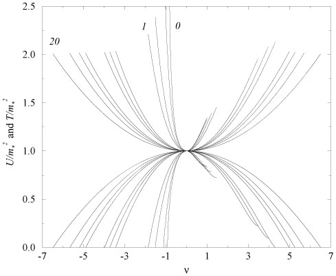
Figure 1.9. Variation of the equation of state with the electromagnetic self-correction q2. It relates the energy per unit length U (upper set of curves) and the tension T (lower set of curves), both in units of m*2, the current-carrier mass, and is plotted against , which is the (sign preserving) square root of the state parameter w. Values used for this correction are in the set [0, 0.1, 0.5, 1, 2, 5, 7, 8, 9, 10, 20], and the figure is calculated for = (m / m*)2 = 1. Increasing the value of q2 enlarges the corresponding curve in such a way that for very large values (in this particular example, it is for for q2 7), the tension on the magnetic side becomes negative before saturation is reached [Gangui, Peter & Boehm, 1998].