3.4. Macroscopic string description

Let us recapitulate briefly the microphysics setting before we see its connection with the macroscopic string description we will develop below. We consider a Witten-type bosonic superconductivity model in which the fundamental Lagrangian is invariant under the action of a U(1) × U(1) symmetry group. The first U(1) is spontaneously broken through the usual Higgs mechanism in which the Higgs field acquires a non-vanishing vacuum expectation value. Hence, at an energy scale m_s ~ ^1/2 (we will call m_s = m hereafter) we are left with a network of ordinary cosmic strings with tension and energy per unit length T ~ U ~ m², as dictated by the Kibble mechanism.

The Higgs field is coupled not only with its associated gauge vector but also with a second charged scalar boson , the current carrier field, which in turn obeys a quartic potential. A second phase transition breaks the second U(1) gauge (or global, in the case of neutral currents) group and, at an energy scale ~ m_*, the generation of a current-carrying condensate in the vortex makes the tension no longer constant, but dependent on the magnitude of the current, with the general feature that T m² U, breaking therefore the degeneracy of the Nambu-Goto strings (more below). The fact that || 0 in the string results in that either electromagnetism (in the case that the associated gauge vector A⁽⁾_µ is the electromagnetic potential) or the global U(1) is spontaneously broken in the core, with the resulting Goldstone bosons carrying charge up and down the string.

Macroscopic quantities

So, let us define the relevant macroscopic quantities needed to find the string equation of state. For that, we have to first express the energy momentum tensor as follows

(33)

One then calculates the macroscopic quantities internal to the string worldsheet (recall `internal' means coordinates t,z)

(34)

The macroscopic charge density/current intensity is defined as

(35)

Now, the state parameter is sgn(w) |w|^1/2. For vanishing coupling e we have w ~ k² - ² and yields the energy of the carrier (in the case w < 0) or its momentum (w > 0).

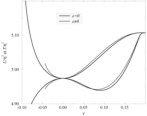
We get the energy per unit length U and the tension of the string T by diagonalizing ^ab

(36)

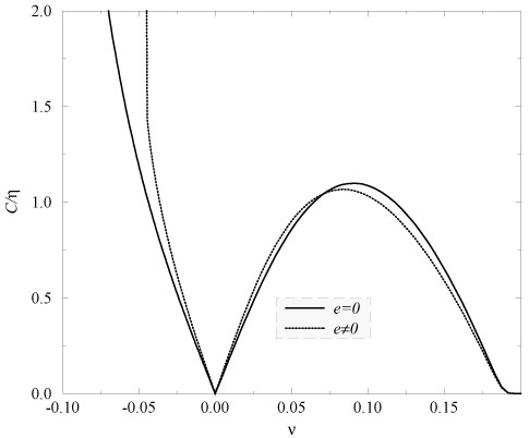
Figure 1.8. Variation of the relevant macroscopic quantities with the state parameter. In the left panel we show the variation of the amplitude of the macroscopic (integrated) charge density (for w < 0) and current intensity (for w > 0) along the string core versus the state parameter, as defined by sgn(w)|w|1/2. In the right panel one can see the corresponding variations of the integrated energy per unit length (upper set of curves) and tension (lower set of curves) for the string. Both the neutral (e = 0) and the charged cases are shown with, in the latter case, a rather exaggerated value of the coupling, in order to distinguish the curves in each set [Peter, 1992].

As shown in Figure (1.8) the general string dynamics in the neutral case does not get much modified when the electromagnetic e-coupling is included. Nevertheless, a couple of main features are worth to note:

• In the magnetic regime there is saturation. In this situation (w > 0) the current intensity C reaches a maximum value and, at the same time, T passes through a minimum.
• In the electric regime there is a phase frequency threshold. In this case (w < 0) the charge density of the conducting string diverges C and the tension tends to vanish T 0⁺. An analytic treatment shows that C (w + m ²)^-1, with m² = 2 f (² - v²). Note that this threshold changes with the coupling, when e is very large.
• We always find T > 0 in w > 0 case. Hence, there is no place for springs, a conjecture first announced by Peter [1993]. Note that T diminishes just a few percent, and then the current saturates. If this were not the case, c²_T = T / U would be negative and this would imply instabilities [Carter, 1989]. Hence, there would be no static equilibrium configurations.

Macroscopic description

Now, let us focus on the macroscopic string description. For a local U(1) we have

(37)

[to stick to usual notation in the literature, we are now changing e - e in our expressions of previous sections]. In this equation we have the conserved Noether current

(38)

Now, recall that A_µ⁽⁾ varies little inside the core, as the penetration depth was bigger than the string core radius. We can then integrate to find the macroscopic current

(39)

which is well-defined even for electromagnetic coupling e 0.

The macroscopic dynamics is describable in terms of a Lagrangian function (w) depending only on the internal degrees of freedom of the string. Now it is 's gradient that characterizes local state of string through

(40)

where _ab is the induced metric on the worldsheet. The latter is given in terms of the background spacetime metric g_µ with respect to the 4-dimensional background coordinates x^µ of the worldsheet. We use a comma to denote simple partial differentiation with respect to the worldsheet coordinates ^a and using Latin indices for the worldsheet coordinates ^₁ = (spacelike), ^₀ = (timelike). As we saw above, the gauge covariant derivative _|a is expressible in the presence of a background electromagnetic field with Maxwellian gauge covector A_µ⁽⁾ (A_µ hereafter) by _|a = _{, a} - eA_µ x^µ_,a. So, now a key rôle is played by the squared of the gradient of in characterizing the local state of the string through w.

The dynamics of the system is determined by the Lagrangian (w). Note there is no explicit appearance of in . From it we get the conserved particle current vector z_a, such that

(41)

Let's define -d / dw = ¹/₂ ^-1. Matching Eqns. (41) and (39), viz. z_a (macro) I_a (micro) we find

(42)

which allows us to see the interpretation of the quantity ^-1. In fact, we have ^-1 amplitude of -condensate. When w 0 (null) we have 1. (with ₀ the zero current limit of ).