


5.1. CMB power spectrum from strings
The narrow main peak and the presence of the second and the third peaks in the CMB angular power spectrum, as measured by BOOMERANG, MAXIMA and DASI [de Bernardis, et al., 2000; Hanany, et al., 2000; Halverson, et al., 2001], is an evidence for coherent oscillations of the photon-baryon fluid at the beginning of the decoupling epoch [see, e.g., Gangui, 2001]. While such coherence is a property of all passive model, realistic cosmic string models produce highly incoherent perturbations that result in a much broader main peak. This excludes cosmic strings as the primary source of density fluctuations unless new physics is postulated, e.g. models with a varying speed of light [Avelino & Martins, 2000]. In addition to purely active or passive models, it has been recently suggested that perturbations could be seeded by some combination of the two mechanisms. For example, cosmic strings could have formed just before the end of inflation and partially contributed to seeding density fluctuations. It has been shown [Contaldi, et al., 1999; Battye & Weller, 2000; Bouchet, et al., 2001] that such hybrid models can be rather successful in fitting the CMB power spectrum data.
Calculating CMB anisotropies sourced by topological defects is a rather difficult task. In inflationary scenario the entire information about the seeds is contained in the initial conditions for the perturbations in the metric. In the case of cosmic defects, perturbations are continuously seeded over the period of time from the phase transition that had produced them until today. The exact determination of the resulting anisotropy requires, in principle, the knowledge of the energy-momentum tensor [or, if only two point functions are being calculated, the unequal time correlators, Pen, Seljak, & Turok, 1997] of the defect network and the products of its decay at all times. This information is simply not available! Instead, a number of clever simplifications, based on the expected properties of the defect networks (e.g. scaling), are used to calculate the source. The latest data from BOOMERANG and MAXIMA experiments clearly disagree with the predictions of these simple models of defects [Durrer, Gangui & Sakellariadou, 1996].
The shape of the CMB angular power spectrum is determined by three
main factors: the geometry of the universe, coherence and causality.
The curvature of the universe directly affects the paths of light rays
coming to us from the surface of last scattering. In a closed
universe, because of the lensing effect induced by the positive
curvature, the same physical distances between points on the sky would
correspond to larger angular scales. As a result, the peak structure
in the CMB angular power spectrum would shift to larger angular scales
or, equivalently, to smaller values of the multipoles
 's.
's.
The prediction of the cosmic string model of
[Pogosian & Vachaspati,
1999]
for  total =
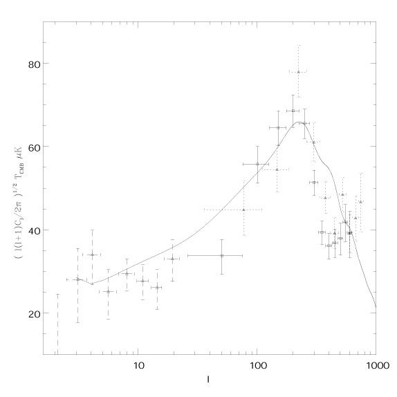
1.3 is shown in Figure 1.14. As can be seen,
the main peak in the angular power spectrum can be
matched by choosing a reasonable value for
total. However, even with the main peak in the
right place the
agreement with the data is far from satisfactory. The peak is
significantly wider than that in the data and there is no sign of a
rise in power at l
total =
1.3 is shown in Figure 1.14. As can be seen,
the main peak in the angular power spectrum can be
matched by choosing a reasonable value for
total. However, even with the main peak in the
right place the
agreement with the data is far from satisfactory. The peak is
significantly wider than that in the data and there is no sign of a
rise in power at l
 600 as the actual
data seems to suggest
[Hanany, et al., 2000].
The sharpness and the height of the main peak
in the angular spectrum can be enhanced by including the effects of
gravitational radiation
[Contaldi, Hindmarsh &
Magueijo, 1999]
and wiggles
[Pogosian & Vachaspati,
1999].
More precise high-resolution numerical simulations of
string networks in realistic cosmologies with a large contribution
from
600 as the actual
data seems to suggest
[Hanany, et al., 2000].
The sharpness and the height of the main peak
in the angular spectrum can be enhanced by including the effects of
gravitational radiation
[Contaldi, Hindmarsh &
Magueijo, 1999]
and wiggles
[Pogosian & Vachaspati,
1999].
More precise high-resolution numerical simulations of
string networks in realistic cosmologies with a large contribution
from  are needed to
determine the exact amount of
small-scale structure on the strings and the nature of the products of
their decay. It is, however, unlikely that including these effects
alone would result in a sufficiently narrow main peak and some
presence of a second peak.
are needed to
determine the exact amount of
small-scale structure on the strings and the nature of the products of
their decay. It is, however, unlikely that including these effects
alone would result in a sufficiently narrow main peak and some
presence of a second peak.
|
Figure 1.14. The CMB power spectrum
produced by the wiggly string model of
[Pogosian &
Vachaspati, 1999]
in a closed universe with
|
This brings us to the issues of causality and coherence and how the random nature of the string networks comes into the calculation of the anisotropy spectrum. Both experimental and theoretical results for the CMB power spectra involve calculations of averages. When estimating the correlations of the observed temperature anisotropies, it is usual to compute the average over all available patches on the sky. When calculating the predictions of their models, theorists find the average over the ensemble of possible outcomes provided by the model.
In inflationary models, as in all passive models, only the initial conditions for the perturbations are random. The subsequent evolution is the same for all members of the ensemble. For wavelengths higher than the Hubble radius, the linear evolution equations for the Fourier components of such perturbations have a growing and a decaying solution. The modes corresponding to smaller wavelengths have only oscillating solutions. As a consequence, prior to entering the horizon, each mode undergoes a period of phase "squeezing" which leaves it in a highly coherent state by the time it starts to oscillate. Coherence here means that all members of the ensemble, corresponding to the same Fourier mode, have the same temporal phase. So even though there is randomness involved, as one has to draw random amplitudes for the oscillations of a given mode, the time behavior of different members of the ensemble is highly correlated. The total spectrum is the ensemble-averaged superposition of all Fourier modes, and the predicted coherence results in an interference pattern seen in the angular power spectrum as the well-known acoustic peaks.
In contrast, the evolution of the string network is highly
non-linear. Cosmic strings are expected to move at relativistic
speeds, self-intersect and reconnect in a chaotic fashion. The
consequence of this behavior is that the unequal time correlators of
the string energy-momentum vanish for time differences larger than a
certain coherence time
( c in
Figure 1.15). Members of
the ensemble corresponding to a given mode of perturbations will have
random temporal phases with the "dice" thrown on average once in
each coherence time. The coherence time of a realistic string network
is rather short. As a result, the interference pattern in the angular
power spectrum is completely washed out.
c in
Figure 1.15). Members of
the ensemble corresponding to a given mode of perturbations will have
random temporal phases with the "dice" thrown on average once in
each coherence time. The coherence time of a realistic string network
is rather short. As a result, the interference pattern in the angular
power spectrum is completely washed out.
Causality manifests itself, first of all, through the initial
conditions for the string sources, the perturbations in the metric and
the densities of different particle species. If one assumes that the
defects are formed by a causal mechanism in an otherwise smooth
universe then the correct initial condition are obtained by setting
the components of the stress-energy pseudo-tensor
µ to zero
[Veeraraghavan &
Stebbins, 1990;
Pen, Spergel & Turok,
1994].
These are the same as the isocurvature initial conditions
[Hu, Spergel & White,
1997].
A generic prediction of isocurvature models
(assuming perfect coherence) is that the first acoustic peak is almost
completely hidden. The main peak is then the second acoustic peak and
in flat geometries it appears at
300 - 400. This is due to
the fact that after entering the horizon a given Fourier mode of the
source perturbation requires time to induce perturbations in the
photon density.
Causality also implies that no superhorizon correlations in the
string energy density are allowed. The correlation length of a
"realistic" string network is normally between 0.1 and 0.4 of the
horizon size.
to zero
[Veeraraghavan &
Stebbins, 1990;
Pen, Spergel & Turok,
1994].
These are the same as the isocurvature initial conditions
[Hu, Spergel & White,
1997].
A generic prediction of isocurvature models
(assuming perfect coherence) is that the first acoustic peak is almost
completely hidden. The main peak is then the second acoustic peak and
in flat geometries it appears at
300 - 400. This is due to
the fact that after entering the horizon a given Fourier mode of the
source perturbation requires time to induce perturbations in the
photon density.
Causality also implies that no superhorizon correlations in the
string energy density are allowed. The correlation length of a
"realistic" string network is normally between 0.1 and 0.4 of the
horizon size.
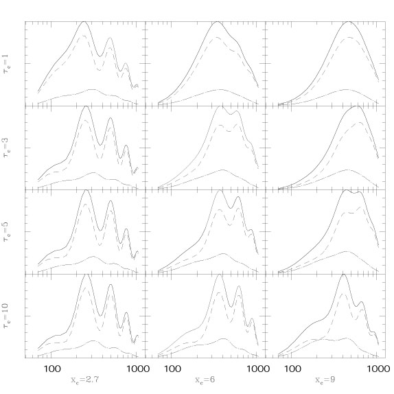
An interesting study was performed by Magueijo, Albrecht, Ferreira & Coulson [1996], where they constructed a toy model of defects with two parameters: the coherence length and the coherence time. The coherence length was taken to be the scale at which the energy density power spectrum of the strings turns from a power law decay for large values of k into a white noise at low k. This is essentially the scale corresponding to the correlation length of the string network. The coherence time was defined in the sense described in the beginning of this section, in particular, as the time difference needed for the unequal time correlators to vanish. Their study showed (see Figure 1.15) that by accepting any value for one of the parameters and varying the other (within the constraints imposed by causality) one could reproduce the oscillations in the CMB power spectrum. Unfortunately for cosmic strings, at least as we know them today, they fall into the parameter range corresponding to the upper right corner in Figure 1.15.
|
Figure 1.15. The predictions of the toy
model of
Magueijo, et al. [1996]
for different values of parameters xc, the
coherence length, and
|
In order to get a better fit to present-day observations, cosmic strings must either be more coherent or they have to be stretched over larger distances, which is another way of making them more coherent. To understand this imagine that there was just one long straight string stretching across the universe and moving with some given velocity. The evolution of this string would be linear and the induced perturbations in the photon density would be coherent. By increasing the correlation length of the string network we would move closer to this limiting case of just one long straight string and so the coherence would be enhanced.
The question of whether or not defects can produce a pattern of the CMB power spectrum similar to, and including the acoustic peaks of, that produced by the adiabatic inflationary models was repeatedly addressed in the literature [Contaldi, Hindmarsh & Magueijo 1999; Magueijo, et al. 1996; Liddle, 1995; Turok, 1996; Avelino & Martins, 2000]. In particular, it was shown [Magueijo, et al. 1996; Turok, 1996] that one can construct a causal model of active seeds which for certain values of parameters can reproduce the oscillations in the CMB spectrum. The main problem today is that current realistic models of cosmic strings fall out of the parameter range that is needed to fit the observations. At the moment, only the (non-minimal) models with either a varying speed of light or hybrid contribution of strings+inflation are the only ones involving topological defects that to some extent can match the observations. One possible way to distinguish their predictions from those of inflationary models would be by computing key non-Gaussian statistical quantities, such as the CMB bispectrum.

 /
/
 c(
c(