5.4. CMB polarization

The possibility that the CMB be polarized was first discussed by Martin Rees in 1968, in the context of anisotropic Universe models. In spite of his optimism, and after more than thirty years, there is still no positive detection of the polarization field. Unlike the BOOMERANG Œ [G experiment, MAP will have the capability to detect it and this to a level of better than 10 µK in its low frequency channels. Polarization is an important probe both for cosmological models and for the more recent history of our nearby Universe. It arises from the interactions of CMB photons with free electrons; hence, polarization can only be produced at the last scattering surface (its amplitude depends on the duration of the decoupling process) and, unlike temperature fluctuations, it is unaffected by variations of the gravitational potential after last scattering. Future measurements of polarization will thus provide a clean view of the inhomogeneities of the Universe at about 400,000 years after the Bang.

For understanding polarization, a couple of things should be clear. First, the energy of the photons is small compared to the mass of the electrons. Then, the CMB frequency does not change, since the electron recoil is negligible. Second, the change in the CMB polarization (i.e., the orientation of the oscillating electric field of the radiation) occurs due to a certain transition, called Thomson scattering. The transition probability per unit time is proportional to a combination of the old (ⁱⁿ) and new (^out) directions of polarization in the form |ⁱⁿ·^out|². In other words, the initial direction of polarization will be favored. Third, an oscillating will push the electron to also oscillate; the latter can then be seen as a dipole (not to be confused with the CMB dipole), and dipole radiation emits preferentially perpendicularly to the direction of oscillation. These `rules' will help us understand why the CMB should be linearly polarized.

Previous to the recombination epoch, the radiation field is unpolarized. In unpolarized light the electric field can be decomposed into the two orthogonal directions (along, say, and perpendicular to the line of propagation (). The electric field along ⁱⁿ (suppose is vertical) will make the electron oscillate also vertically. Hence, the dipolar radiation will be maximal over the horizontal xy-plane. Analogously, dipole radiation due to the electric field along will be on the yz-plane. If we now look from the side (e.g., from , on the horizontal plane and perpendicularly to the incident direction ) we will see a special kind of scattered radiation. From our position we cannot perceive the radiation that the electron oscillating along the direction would emit, just because this radiation goes to the yz-plane, orthogonal to us. Then, it is as if only the vertical component (ⁱⁿ) of the incoming electric field would cause the radiation we perceive. From the above rules we know that the highest probability for the polarization of the outgoing radiation ^out will be to be aligned with the incoming one ⁱⁿ, and therefore it follows that the outgoing radiation will be linearly polarized. Now, as both the chosen incoming direction and our position as observers were arbitrary, the result will not be modified if we change them. Thomson scattering will convert unpolarized radiation into linearly polarized one.

This however is not the end of the story. To get the total effect we need to consider all possible directions from which photons will come to interact with the target electron, and sum them up. We see easily that for an initial isotropic radiation distribution the individual contributions will cancel out: just from symmetry arguments, in a spherically symmetric configuration no direction is privileged, unlike the case of a net linear polarization which would select one particular direction.

Fortunately, we know the CMB is not exactly isotropic; to the millikelvin precision the dominant mode is dipolar. So, what about a CMB dipolar distribution ? Although spatial symmetry does not help us now, a dipole will not generate polarization either. Take, for example, the radiation incident onto the electron from the left to be more intense than the radiation incident from the right, with average intensities above and below (that's a dipole); it then suffices to sum up all contributions to see that no net polarization survives. However, if the CMB has a quadrupolar variation in temperature (that it has, first discovered by COBE, to tens of µK precision) then there will be an excess of vertical polarization from left- and right-incident photons (assumed hotter than the mean) with respect to the horizontal one from top and bottom light (cooler). From any point of view, orthogonal contributions to the final polarization will be different, leaving a net linear polarization in the scattered radiation.

Within standard recombination models the predicted level of linear polarization on large scales is tiny (see Figure 1.17): the quadrupole generated in the radiation distribution as the photons travel between successive scatterings is too small. Multiple scatterings make the plasma very homogeneous and only wavelengths that are small enough (big 's) to produce anisotropies over the (rather short) mean free path of the photons will lead to a significant quadrupole, and thus also to polarization. Indeed, if the CMB photons last scattered at z ~ 1100, the SCDM model with h = 1 predicts no more than 0.05 µK on scales greater than a few degrees. Hence, measuring polarization represents an experimental challenge. There is still no positive detection and the best upper limits a few years ago were around 25 µK, obtained by Edward Wollack and collaborators in 1993, and now improved to roughly 10µK on subdegree angular scales by Hedman, et al., [2001] ⁽²⁰⁾.

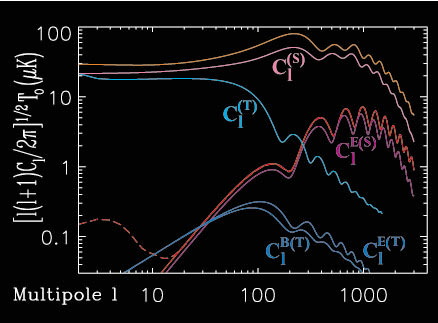
Figure 1.17. CMB Polarization for two different models. Red and orange (unlabeled) curves are the angular spectra derived for a CHDM model, both with (red dashed line) and without (red full line) reionization. The temperature anisotropy spectrum from scalar perturbations (proportional to [ C ]1/2, orange curve) is virtually unchanged for both ionization histories. The polarization spectrum ( [ CE(S) ]1/2, red curves), although indistinguishable for 20, dramatically changes for small 's; in this model the Universe is reionized suddenly at low redshift with optical depth c = 0.05. Blue and violet curves represent a SCDM model but with a high tensor-mode amplitude, T/S = 1 at the quadrupole ( = 2) level, with scale-invariant spectral indices ns = 1 and nT = 0. Separate scalar (noted C(S)) and tensor (C(T)) contributions to temperature anisotropies are shown (top curves). Scalar modes only generate E-type polarization (CE(S)), which is smaller than the corresponding red curve of the CHDM model both due to differences in the models (notably 0 for the red curves) and due to the influence of tensors on the normalization at small . E- and B-type polarization from tensor modes are also shown, respectively CE(T) and CB(T). Model spectra were computed with CMBFAST and are normalized to T = 10 = 27.9µK.

However, CMB polarization increases remarkably around the degree-scale in standard models. In fact, for < 1° a bump with superimposed acoustic oscillations reaching ~ 5 µK is generically forecasted. On these scales, like for the temperature anisotropies, the polarization field shows acoustic oscillations. However, polarization spectra are sharper: temperature fluctuations receive contributions from both density (dominant) and velocity perturbations and these, being out of phase in their oscillation, partially cancel each other. On the other hand, polarization is mainly produced by velocity gradients in the baryon-photon fluid before last scattering, which also explains why temperature and polarization peaks are located differently. Moreover, acoustic oscillations depend on the nature of the underlying perturbation; hence, we do not expect scalar acoustic sound-waves in the baryon-photon plasma, propagating with characteristic adiabatic sound speed c_s ~ c / 3, close to that of an ideal radiative fluid, to produce the same peak-frequency as that produced by gravitational waves, which propagate with the speed of light c (see Fig. 1.17).

The main technical complication with polarization (characterized by a tensor field) is that it is not invariant under rotations around a given direction on the sky, unlike the temperature fluctuation that is described by a scalar quantity and invariant under such rotations. The level of linear polarization is conveniently expressed in terms of the Stokes parameters Q and U. It turns out that there is a clever combination of these parameters that results in scalar quantities (in contrast to the above noninvariant tensor description) but with different transformation properties under spatial inversions (parity transformations). Then, inspired by classical electromagnetism, any polarization pattern on the sky can be separated into `electric' (scalar, unchanged under parity transformation) and `magnetic' (pseudo-scalar, changes sign under parity) components (E- and B-type polarization, respectively).

CMB polarization from global defects

One then expands these different components in terms of spherical harmonics, very much like we did for temperature anisotropies, getting coefficients a^m for E and B polarizations and, from these, the multipoles C^E,B. The interesting thing is that (for symmetry reasons) scalar-density perturbations will not produce any B polarization (a pseudo-scalar), that is C^B(S) = 0. We see then that an unambiguous detection of some level of B-type fluctuations will be a signature of the existence (and of the amplitude) of a background of gravitational waves ! [Seljak & Zaldarriaga, 1997] (and, if present, also of rotational modes, like in models with topological defects).

Linear polarization is a symmetric and traceless 2x2 tensor that requires 2 parameters to fully describe it: Q, U Stokes parameters. These depend on the orientation of the coordinate system on the sky. It is convenient to use Q + iU and Q - iU as the two independent combinations, which transform under right-handed rotation by an angle as (Q + iU)' = e^-2i(Q + iU) and (Q - iU)' = e²ⁱ(Q - iU). These two quantities have spin-weights 2 and -2 respectively and can be decomposed into spin ±2 spherical harmonics _±2Y_lm

(114) (115)

Spin s spherical harmonics form a complete orthonormal system for each value of s. Important property of spin-weighted basis: there exists spin raising and lowering operators ' and ')]. By acting twice with a spin lowering and raising operator on (Q + iU) and (Q - iU) respectively one obtains quantities of spin 0, which are rotationally invariant. These quantities can be treated like the temperature and no ambiguities connected with the orientation of coordinate system on the sky will arise. Conversely, by acting with spin lowering and raising operators on usual harmonics spin s harmonics can be written explicitly in terms of derivatives of the usual spherical harmonics. Their action on _±2Y_lm leads to

(116) (117)

With these definitions the expressions for the expansion coefficients of the two polarization variables become [Seljak & Zaldarriaga, 1997]

(118) (119)

Instead of a_2,lm, a_-2,lm it is convenient to introduce their linear electric and magnetic combinations

(120)

These two behave differently under parity transformation: while E remains unchanged B changes the sign, in analogy with electric and magnetic fields.

To characterize the statistics of the CMB perturbations only four power spectra are needed, those for X = T, E, B and the cross correlation between T and E. The cross correlation between B and E or B and T vanishes because B has the opposite parity of T and E. As usual, the spectra are defined as the rotationally invariant quantities

(121)

in terms of which on has

(122) (123) (124)

According to what was said above, one expects some amount of polarization to be present in all possible cosmological models. However, symmetry breaking models giving rise to topological defects differ from inflationary models in several important aspects, two of which are the relative contributions from scalar, vector and tensor modes and the coherence of the seeds sourcing the perturbation equations. In the local cosmic string case one finds that in general scalar modes are dominant, if one compares to vector and tensor modes in the usual decomposition of perturbations. The situation with global topological defects is radically different and this leads to a very distinctive signature in the polarization field.

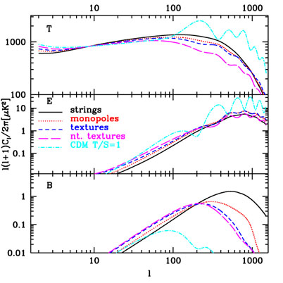
Temperature and polarization spectra for various symmetry breaking models were calculated by Seljak, Pen & Turok [1997] and are shown in figure 1.18. Both electric and magnetic components of polarization are shown for a variety of global defects. They also plot for comparison the corresponding spectra in a typical inflationary model, namely, the standard CDM model (h = 0.5, = 1, _baryon = 0.05) but with equal amount of scalars and tensors perturbations (noted T / S = 1) which maximizes the amount of B component from inflationary models. In all the models they assumed a standard reionization history. The most interesting feature they found is the large magnetic mode polarization, with a typical amplitude of ~ 1 µK on degree scales [exactly those scales probed by Hedman, et al., 2001]. For multipoles below l ~ 100 the contributions from E and B are roughly equal. This differs strongly from the inflationary model predictions, where B is much smaller than E on these scales even for the extreme case of T / S ~ 1. Inflationary models only generate scalar and tensor modes, while global defects also have a significant contribution from vector modes. As we mentioned above, scalar modes only generate E, vector modes predominantly generate B, while for tensor modes E and B are comparable with B being somewhat smaller. Together this implies that B can be significantly larger in symmetry breaking models than in inflationary models.

Figure 1.18. Power spectra of temperature (T), electric type polarization (E) and magnetic type polarization (B) for global strings, monopoles, textures and nontopological textures [taken from Seljak. et al., 1997]. The corresponding spectra for a standard CDM model with T/S = 1 is also shown for comparison. B polarization turns out to be notably larger for all global defects considered if compared to the corresponding predictions of inflationary models on small angular scales.

Recent studies have shown that in realistic models of inflation cosmic string formation seems quite natural in a post-inflationary preheating phase [Tkachev et al., 1998, Kasuya & Kawasaki, 1998]. So, even if the gross features on CMB maps are produced by a standard (e.g., inflationary) mechanism, the presence of defects, most particularly cosmic strings, could eventually leave a distinctive signature. One such feature could be found resorting to CMB polarization: the lens effect of a string on the small scale E-type polarization of the CMB induces a significant amount of B-type polarization along the line-of-sight [Zaldarriaga & Seljak, 1998; Benabed & Bernardeau 2000]. This is an effect analogous to the Kaiser-Stebbins effect for temperature maps.

In the inflationary scenario, scalar density perturbations generate a scalar polarization pattern, given by E -type polarization, while tensor modes have the ability to induce both E and B types of polarization. However, tensor modes contribute little on very small angular scales in these models. So, if one considers, say, a standard CDM model, only scalar primary perturbations will be present without defects. But if a few strings are left from a very early epoch, by studying the patch of the sky where they are localized, a distinctive signature could come to light.

In the small angular scale limit, in real space and in terms of the Stokes parameters Q and U one can express the E and B fields as follows

(125) (126)

The polarization vector is parallel transported along the geodesics. The lens affects the polarization by displacing the apparent position of the polarized light source. Hence, the observed Stokes parameters and are given in terms of the primary (unlensed) ones by: () = Q( + ) and () = U( + ). The displacement is given by the integration of the gravitational potential along the line-of-sights. Of course, here the `potential' acting as lens is the cosmic string whose effect on the polarization field we want to study.

In the case of a straight string which is aligned along the y axis, the deflection angle (or half of the deficit angle) is 4Gµ [Vilenkin & Shellard, 2000] and this yields a displacement _x = ± ₀ with

(127)

with no displacement along the y axis. _lss,s and _s,us are the cosmological angular distances between the last scattering surface and the string, and between the string and us, respectively. They can be computed, in an Einstein-de Sitter universe (critical density, just dust and no ), from

(128)

by taking z₁ = 0 for us and z₂ 1000 for the last scattering surface; see [Bartelmann & Schneider, 2001]. For the usual case in which the redshift of the string z_s is well below the z_lss one has _lss,s / _lss,us 1 / (1 + z_s)^1/2. Taking this ratio of order 1/2 (i.e., distance from us to the last scattering surface equal to twice that from the string to the last scattering surface) yields z_s 3. Plugging in some numbers, for typical GUT strings on has Gµ 10^-6 and so the typical expected displacement is about less than 10 arc seconds. Benabed & Bernardeau [2000] compute the resulting B component of the polarization and find that the effect is entirely due to the discontinuity induced by the string, being nonzero just along the string itself. This clearly limits the observability of the effect to extremely high resolution detectors, possibly post-Planck ones.

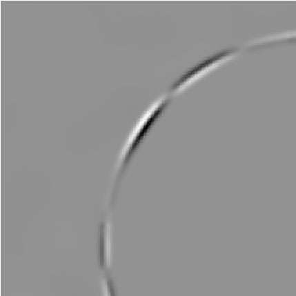
The situation for circular strings is different. As shown by de Laix & Vachaspati [1996] the lens effect of such a string, when facing the observer, is equivalent to the one of a static linear mass distribution. Considering then a loop centered at the origin of the coordinate system, the displacement field can be expressed very simply: observing in a direction through the loop, has to vanish, while outside of the loop the displacement decreases as _l / , i.e., inversely proportional to the angle. One then has [Benabed & Bernardeau, 2000]

(129)

where _l is the loop radius.

This ansatz for the displacement, once plugged into the above equations, yields the B field shown in both panels of Figure 1.19. A weak lensing effect is barely distinguishable outside the string loop, while the strong lensing of those photons traveling close enough to the string is the most clear signature, specially for the high resolution simulation. One can check that the hot and cold spots along the string profile have roughly the same size as for the polarization field in the absence of the string loop. The simulations performed show a clear feature in the maps, although limited to low resolutions this can well be confused with other secondary polarization sources. It is well known that point radio sources and synchrotron emission from our galaxy may contribute to the foreground [de Zotti et al. 1999] and are polarized at a 10% level. Also lensing from large scale structure and dust could add to the problem.

Figure 1.19. Simulations for the B field in the case of a circular loop. The angular size of the figure is 50' × 50'. The resolution is 5' (left) and 1.2' (right). The discontinuity in the B field is sharper the better the resolution. Weak lensing of CMB photons passing relatively apart from the position of the string core are apparent as faint patches outside of the string loop on the left panel. [Benabed & Bernardeau 2000].

²⁰ They actually find upper limits of 14 µK and 13µK on the amplitudes of the E and B modes, respectively, of the polarization field - more below. And, if in their analysis they assumed there are no B modes, then the limit on E improves to 10µK (all limits to 95% confidence level). Back.