5.3. CMB bispectrum from strings

To calculate the sources of perturbations we have used an updated version of the cosmic string model first introduced by Albrecht et al. [1997] and further developed in [Pogosian & Vachaspati, 1999], where the wiggly nature of strings was taken into account. In these previous works the model was tailored to the computation of the two-point statistics (matter and CMB power spectra). When dealing with higher-order statistics, such as the bispectrum, a different strategy needs to be employed.

In the model, the string network is represented by a collection of uncorrelated straight string segments produced at some early epoch and moving with random uncorrelated velocities. At every subsequent epoch, a certain fraction of the number of segments decays in a way that maintains network scaling. The length of each segment at any time is taken to be equal to the correlation length of the network. This and the root mean square velocity of segments are computed from the velocity-dependent one-scale model of Martins & Shellard [1996]. The positions of segments are drawn from a uniform distribution in space, and their orientations are chosen from a uniform distribution on a two-sphere.

The total energy of the string network in a volume V at any time is E = NµL, where N is the total number of string segments at that time, µ is the mass per unit length, and L is the length of one segment. If L is the correlation length of the string network then, according to the one-scale model, the energy density is = E / V = µ/L², where V = V₀ a³, the expansion factor a is normalized so that a = 1 today, and V₀ is a constant simulation volume. It follows that N = V / L³ = V₀ / ³, where = L / a is the comoving correlation length. In the scaling regime l is approximately proportional to the conformal time and so the number of strings N() within the simulation volume V₀ falls as ^-3.

To calculate the CMB anisotropy one needs to evolve the string network over at least four orders of magnitude in cosmic expansion. Hence, one would have to start with N 10¹² string segments in order to have one segment left at the present time. Keeping track of such a huge number of segments is numerically infeasible. A way around this difficulty was suggested in Ref.[3], where the idea was to consolidate all string segments that decay at the same epoch. The number of segments that decay by the (discretized) conformal time _i is

(104)

where n() = [()]^-3 is the number density of strings at time . The energy-momentum tensor in Fourier space, ⁱ_µ, of these N_d(_i) segments is a sum

(105)

where ^im_µ is the Fourier transform of the energy-momentum of the m-th segment. If segments are uncorrelated, then

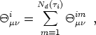
(106)

and

(107)

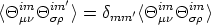
Here the angular brackets < ... > denote the ensemble average, which in our case means averaging over many realizations of the string network. If we are calculating power spectra, then the relevant quantities are the two-point functions of ⁱ_µ, namely

(108)

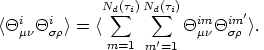
Eq. (106) allows us to write

(109)

where ⁱ¹_µ is of the energy-momentum of one of the segments that decay by the time _i. The last step in Eq. (109) is possible because the segments are statistically equivalent. Thus, if we only want to reproduce the correct power spectra in the limit of a large number of realizations, we can replace the sum in Eq. (105) by

(110)

The total energy-momentum tensor of the network in Fourier space is a sum over the consolidated segments:

(111)

So, instead of summing over _i=1^K N_d(_i) 10¹² segments we now sum over only K segments, making K a parameter.

For the three-point functions we extend the above procedure. Instead of Eqs. (108) and (109) we now write

(112)

Therefore, for the purpose of calculation of three-point functions, the sum in Eq. (105) should now be replaced by

(113)

Both expressions in Eqs. (110) and (113), depend on the simulation volume, V₀, contained in the definition of N_d(_i) given in Eq. (104). This is to be expected and is consistent with our calculations, since this volume cancels in expressions for observable quantities.

Note also that the simulation model in its present form does not allow computation of CMB sky maps. This is because the method of finding the two- and three-point functions as we described involves "consolidated" quantities ⁱ_µ which do not correspond to the energy-momentum tensor of a real string network. These quantities are auxiliary and specially prepared to give the correct two- or three-point functions after ensemble averaging.

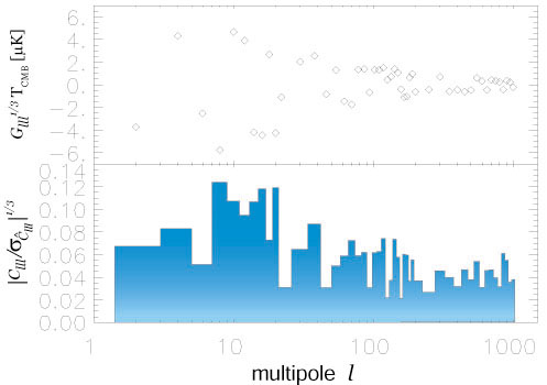
In Fig. 1.16 we show the results for G_lll^1/3 [cf. Eq. (99)]. It was calculated using the string model with 800 consolidated segments in a flat universe with cold dark matter and a cosmological constant. Only the scalar contribution to the anisotropy has been included. Vector and tensor contributions are known to be relatively insignificant for local cosmic strings and can safely be ignored in this model [3, 131] ⁽¹⁸⁾. The plots are produced using a single realization of the string network by averaging over 720 directions of k_i. The comparison of G_lll^1/3 (or equivalently C_lll^1/3) with its cosmic variance [cf. Eq. (101)] clearly shows that the bispectrum (as computed from the present cosmic string model) lies hidden in the theoretical noise and is therefore undetectable for any given value of l.

Let us note, however, that in its present stage the string code employed in these computations describes Brownian, wiggly long strings in spite of the fact that long strings are very likely not Brownian on the smallest scales, as recent field-theory simulations indicate. In addition, the presence of small string loops [Wu, et al., 1998] and gravitational radiation into which they decay were not yet included in this model. These are important effects that could, in principle, change the above predictions for the string-generated CMB bispectrum on very small angular scales.

Figure 1.16. The CMB angular bispectrum in the `diagonal' case (Glll1/3) from wiggly cosmic strings in a spatially flat model with cosmological parameters CDM = 0.3, baryon = 0.05, = 0.65, and Hubble constant H = 0.65 km s-1 Mpc-1 [upper panel]. In the lower panel we show the ratio of the signal to theoretical noise |Clll / lll|1/3 for different multipole indices. Normalization follows from fitting the power spectrum to the BOOMERANG and MAXIMA data.

As the universe becomes transparent, strings continue to leave their imprint on the CMB mainly due to the Kaiser & Stebbins [1984] effect. As we mentioned in previous sections, this effect results in line discontinuities in the temperature field of photons passing on opposite sides of a moving long string. ⁽¹⁹⁾ However, this effect can result in non-Gaussian perturbations only on sufficiently small scales. This is because on scales larger than the characteristic inter-string separation at the time of the radiation-matter equality, the CMB temperature perturbations result from superposition of effects of many strings and are likely to be Gaussian. Avelino et al. [1998] applied several non-Gaussian tests to the perturbations seeded by cosmic strings. They found the density field distribution to be close to Gaussian on scales larger than 1.5 (_M h²)^-1 Mpc, where _M is the fraction of cosmological matter density in baryons and CDM combined. Scales this small correspond to the multipole index of order l ~ 10⁴.

¹⁸ The contribution of vector and tensor modes is large in the case of global strings [Turok, Pen & Seljak, 1998; Durrer, Gangui & Sakellariadou, 1996]. Back.

¹⁹ The extension of the Kaiser-Stebbins effect to polarization will be treated below. In fact, Benabed and Bernardeau [2000] have recently considered the generation of a B-type polarization field out of E-type polarization, through gravitational lensing on a cosmic string. Back.