


Several, more or less independent, ways of measuring the position and inclination angles, of galaxies have been proposed and used so far:
i) Large-scale kinematics. Assuming that the emitting material is in a thin planar disk and is in circular motion around the center of the galaxy, one can minimize, e.g. by least squares, the departures from such a flow (Warner et al. 1973). This method is well adapted to HI velocity fields, provided the galaxy is not too perturbed, and has been widely used in such studies (e.g. Bosma 1981). If the above mentioned assumptions are met, it is the safest of all methods, at least as far as the P.A. is concerned, since it involves data from all the surface of the galaxy and it is not too hindered by noise. This method has been lately (e.g. Pence et al. 1990) applied to optical data which present a sufficiently good coverage of the surface of the galaxy.
ii) From photometry the position and inclination angles are measured traditionally by fitting ellipses to the outermost isophotes which are not too perturbed by noise and background (e.g. Boroson, 1981, etc).
iii) Grosbol (1985, hereafter G85) used a variant of the above method. He applied one dimensional Fourier transforms to the intensity distribution in the outer parts and adopted the deprojection angles that minimised the bisymmetric Fourier component.
iv) Kent (1985) used the photometric data all through the galaxy and did not limit himself to the outer parts. He assumed that the galaxy consists of two components, a bulge and a disk, the former being considered spherical, and fitted the intensity profiles on the major and minor axes.
v) Iye et al. (1982) calculated the projection angles of NGC 4254 by maximizing the power in the axisymmetric component of the deprojected intensity distribution.
vi) Considére & Athanassoula (1988, hereafter CA88) used the m = 2 spectrum to ensure that there was no contribution from a wrongly deprojected disk and that the signal of the spiral stood out well.
vii) Another method related to the above one consists of plotting the
positions of the HII regions in a
log(r) -  plane
and fitting a straight line to
the arms, thus ensuring that the spirals are logarithmic.
plane
and fitting a straight line to
the arms, thus ensuring that the spirals are logarithmic.
viii) Danver (1942, hereafter D42) obtained visual estimates for 202 galaxies by rotating their images with the help of a special display table, until the galaxy image was circular.
The methods of Iye et al., Considére & Athanassoula, and Danver, i.e. methods v, vi and viii, can be suitably modified so as to apply to HII region distributions. We have refrained from applying method viii, because it is highly subjective, although in the discussion of the individual galaxies that follows, in a few cases, when discordant values are found by the various methods, we will make note of which values gave more reasonable looking results. Method vi necessitates a clear spiral structure, giving a clear signal-to-noise ratio in the m = 2 spectrum. This is often the case when the whole image of the galaxy is being analysed, but seldom in an HII region distribution. Considére & Athanassoula (1982) have already applied it to the HII region distribution of M51 and given a discussion on the results. We have not used this method since very few galaxies in our sample have a spiral structure as clearly delineated as that of M51.
Finally method v cannot be applied as such but rather as described in
the previous section.
It will be referred to hereafter as our first method. It can of course
be applied only to
galaxies whose HII region distribution delineates the axisymmetric
component. If the
HII regions are found only in the spiral arms, i.e. their distribution
delineates mainly
some m > 0 component, another method should be applied (see next
paragraph). Thus all galaxies marked by a Y in Column 6 of
Table 1 were found difficult, or
impossible to
analyse by our first method. Its main disadvantage is that, depending on
whether one uses the density, mass or any other form
r
 (r,
), one
gives more or less weight to the
inner compared to the outer parts of the distribution. Giving weight to
the inner parts
should give wrong results in the case of B or AB galaxies (respectively
8 and 28 galaxies
in our sample according to the RC2), and could falsify the results for
galaxies with a
slight oval component, if this was reflected in the HII region
distribution. Favouring the
outer parts does not seem to introduce any obvious biases, but could
introduce errors in galaxies with asymmetric outer parts.
(r,
), one
gives more or less weight to the
inner compared to the outer parts of the distribution. Giving weight to
the inner parts
should give wrong results in the case of B or AB galaxies (respectively
8 and 28 galaxies
in our sample according to the RC2), and could falsify the results for
galaxies with a
slight oval component, if this was reflected in the HII region
distribution. Favouring the
outer parts does not seem to introduce any obvious biases, but could
introduce errors in galaxies with asymmetric outer parts.
We have thus deviced another method, which we will hereafter refer to as our second method, which does not present the above problem. If we cut an axially symmetric galaxy into N equal sectors, like parts of a cake, then each part should have a roughly equal number of HII regions, but these sectors are not equal in a projected galaxy, and the size of each sector depends on the values of PA and IA. For given values of PA and IA we can deproject the HII region distribution, cut the surface into sectors and then count the HII regions falling in each sector. If the deprojection angles chosen are the correct values, the number in each division must be roughly equal and the dispersion around the mean minimal. Thus the correct PA and IA should minimize the dispersion of the number of HII regions in each angular slice from this mean value. Of course this method will not work for the case of strongly barred galaxies and will present more than one minimum in the (PA, IA) plane in the case of ovals, spirals or other structures. Mercifully, most of the time, these minima are relatively wide apart, so that visual inspection of the deprojected distribution or a very rough knowledge of the deprojection angles are enough to tell the relevant minimum. We have also tried to eliminate the effect of asymmetries by adding the contents of two sectors which are symmetric with respect to the center. An important advantage of this method is that the calculations require very little computing time compared to the first method.
We have tested our second method with the help of many random number realisations of axisymmetric inclined disks. We found that this method, like most others, works better with more inclined galaxies than with less inclined ones since for the former the PA stands out better. Of course the larger the number of points the better the method works. It also works less well for very centrally concentrated distributions or distributions having most regions in the outer parts, i.e. the method favours more uniform coverages.
For most of our test, we used an N(r) = r e-r profile which, as will be shown in a forthcoming paper, is a realistic representation of the HII region number distribution in a fair fraction of galaxies. Realisations with a relatively large number of points have a minimum in the (PA, IA) plane clearly showing the correct values of the deprojection angles. For a low number of points, i.e. less than 200, one often gets more than one minimum. Since many of our galaxies have less than 200 catalogued HII regions, we have made tests to assess the possibilities of the method in such cases. Fifty different realisations of 150 points were made and projected with PA = 120° and IA = 60°. Our second method was then applied to each of them. In 37 realisations the primary minimum was within ± 5° from the right position, and in 47 within ± 10°. The mean for the PA values for the primary minimum is 120° ± 6°, and for the inclination angle 59° ± 5°. We repeated this for an inclination of 45° which, as discussed above, is less favourable to this method. We found a mean of 122° ± 13° and 43° ± 7° for the primary minima.
We applied the same test to our first method, but now with forty realisations of each distribution since this method is more CPU intensive. In all cases there was only one minimum, however it corresponded to values of the PA and IA further away, in the mean, from the correct values than those predicted by the second method. When the correct values were PA = 120° and IA = 60°, it gave PA = 118° ± 9° and IA = 59° + 6°. Similarly for PA = 120° and IA = 45° it gave PA = 122° ± 20° and IA = 46° ± 9°.
These tests gave an estimate of the expected errors in the case of an
axisymmetric
distribution of points. However we expect bigger errors in the cases
where a considerable
number of points are in a spiral. Furthermore the influence of the
spiral structure on the
errors might be different for the two methods. In order to test this we
made 10 different
realisations of two "spiral" galaxies. In the first case 100 points were
drawn from an
axisymmetric distribution and 50 were in spiral component. The numbers
were inversed in the
second case. Initially we tried drawing numbers from a spiral with a
cos 2 component and
a reasonable radial distribution. However this gave a spiral structure
which was too broad and not at all reminiscent of the distribution shown
e.g. in Figure 3. We thus discarded this as
unrealistic and preferred to generate the spiral as follows. We placed
the points initially
equidistantly on a logarithmic spiral with pitch angle
i = 15° and then gave to each of them
two random nudges, in x and y, between 0 and 0.1 times the
maximum radius of the axisymmetric
distribution. The result of this ad hoc method looks much more
realistic than that of the
previous one. Since the amplitude of the spiral does not decrease with
radius in these examples,
we expected, and got, an important Stocke's effect
(Stocke 1955).
However, as there are
distributions of HII regions with this characteristic and since these
were often amidst the
most difficult to treat, we have thought it realistic to leave this
effect in the random
distribution as well. We then applied the same test as above to these
two test distributions
and found, as expected, bigger deviations in the mean from the correct
value than before.
| 
|
| 
|
| 
|
| 
|
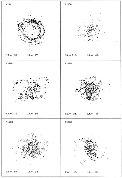
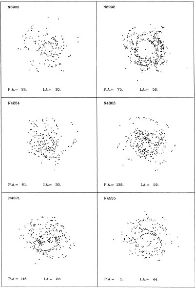
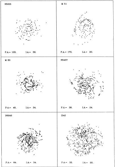
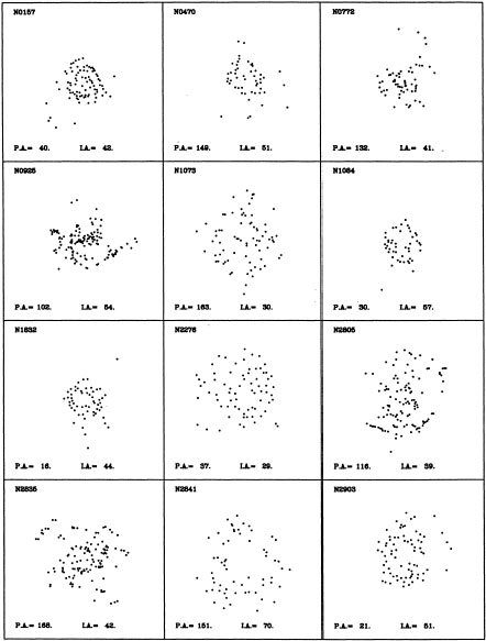
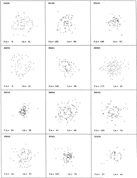
Figure 3. Deprojected HII region distributions of all galaxies in our sample. | |
The first method was, in general, more affected by the nonaxisymmetry of the distribution than the second one. Thus for 10 realisations with 100 points in the disc and 50 in the spiral we obtained for the first method PA = 129° ± 6° and IA = 60° ± 3°, and for the second PA = 122° ± 7° and IA = 49° ± 5°, instead of the correct 120° and 45°. However the values of the departure depend not only on the ratio of points in the spiral to that in the disc, but also on the phase of the spiral with respect to the adopted PA. Thus the values we have given are only indicative.
With the help of the computerised bibliography of the Centre de Données Stellaires in Starsbourg (France) we made a literature search for the PAs and IAs obtained by other methods. Most galaxies had several independent determinations, but not all were judged to be equally reliable.
Our results are summarized in Table 3. The name
of the galaxy is given in Column 1. An I in
Column 2 means that the HII region distribution is irregular, and a II
that it is very
irregular. Columns 3 and 4 give the PA and IA obtained by our first
method (similar to Iye et al.'s method) and Column 6 the step in degrees
( PA,
IA) used in the
partitioning and scanning of the (PA, IA) plane when searching for the
minimum. Column 5 gives the weight
we have assigned to this result. The values of the PA and IA obtained
from our second method
are given in Columns 7 and 8 and the weight we have assigned to this
result in Column 9.
A 20, or 40 in Column 10 means that the galaxies were divided into 20,
respectively 40, equal
sectors. An * was put in Column 11 when the adopted minimum was not the
deepest but a secondary one. For this method the angles
PA and
IA
which we used when looking for the
minima were always 5°. Thus the error bars of the values we
have determined are at
least half this step, or half the number given in Column 6 for our first
method. However they
can be considerably higher if certain structures or associations of
points interfere with
our methods. In Columns 12 and 13 we give the weighted means of the PAs
and IAs obtained by means of our two methods.
PA,
IA) used in the
partitioning and scanning of the (PA, IA) plane when searching for the
minimum. Column 5 gives the weight
we have assigned to this result. The values of the PA and IA obtained
from our second method
are given in Columns 7 and 8 and the weight we have assigned to this
result in Column 9.
A 20, or 40 in Column 10 means that the galaxies were divided into 20,
respectively 40, equal
sectors. An * was put in Column 11 when the adopted minimum was not the
deepest but a secondary one. For this method the angles
PA and
IA
which we used when looking for the
minima were always 5°. Thus the error bars of the values we
have determined are at
least half this step, or half the number given in Column 6 for our first
method. However they
can be considerably higher if certain structures or associations of
points interfere with
our methods. In Columns 12 and 13 we give the weighted means of the PAs
and IAs obtained by means of our two methods.
| Name | First. | Second. | HII. | Bibliography. | Adopted. | |||||||||||||||
| (1) | (2) | (3) | (4) | (5) | (6) | (7) | (8) | (9) | (10) | (11) | (12) | (13) | (14) | (15) | (16) | (17) | (18) | (19) | (20) | (21) |
| N0157 | 46. | 40. | 2 | 2 | 40. | 40. | 1 | 20 | * | 44. | 40. | 35. | 45. | 2 | 1 | 40. | 6. | 42. | 3. | |
| N0224 | 38. | 77. | 3 | 2 | 38. | 77. | 2 | 40 | 38. | 77. | 38. | 77. | 5 | 6 | 38. | 0. | 77. | 0. | ||
| N0300 | 99. | 28. | 0 | 2 | 120. | 60. | 2 | 20 | 120. | 60. | 108. | 45. | 3 | 2 | 110. | 5. | 47. | 7. | ||
| 106. | 42. | 3 | 42 | |||||||||||||||||
| 110. | 43. | 2 | 8 | |||||||||||||||||
| N0470 | I | 144. | 46. | 1 | 2 | 150. | 50. | 2 | 20 | 148. | 49. | 151. | 55. | 2 | 1 | 149. | 3. | 51. | 4. | |
| N0598 | I | 35. | 55. | 1 | 20 | * | 35. | 55. | 22. | 54. | 5 | 48 | 24. | 4. | 55. | 2. | ||||
| 23. | 54. | 3 | 54 | |||||||||||||||||
| 23. | 58. | 2 | 8 | |||||||||||||||||
| N0628 | 160. | 25. | 0 | 2 | 25. | 15. | 1 | 20 | * | 25. | 15. | 25. | 6. | 5 | 50 | 23. | 6. | 8. | 5. | |
| 0. | 0,1 | 7 | ||||||||||||||||||
| 84. | 21. | 0,1 | 1 | |||||||||||||||||
| 26. | 6. | 5 | 54 | |||||||||||||||||
| 10. | 15. | 2 | 8 | |||||||||||||||||
| N0772 | II | 148. | 40. | 1 | 2 | 135. | 40. | 2 | 20 | 139. | 40. | 120. | 43. | 2 | 1 | 132. | 12. | 41. | 2. | |
| N0925 | I | 89. | 63. | 0 | 2 | 95. | 70. | 0 | 20 | 102. | 53. | 4 | 3 | 102. | 1. | 54. | 3. | |||
| 104. | 60. | 1 | 1 | |||||||||||||||||
| N1073 | 168. | 43. | 2 | 2 | 155. | 30. | 2 | 20 | 162. | 37. | 23. | 29. | 0,2 | 1 | 163. | 5. | 30. | 9. | ||
| 164. | 19. | 4,2 | 34 | |||||||||||||||||
| N1084 | 26. | 66. | 1 | 2 | 30. | 50. | 1 | 20 | * | 28. | 58. | 31. | 55. | 2 | 4 | 30. | 2. | 57. | 7. | |
| N1232 | 84. | 26. | 1 | 2 | 85. | 30. | 2 | 20 | 85. | 29. | 87. | 39. | 2 | 1 | 86. | 1. | 33. | 6. | ||
| N1313 | I | 20. | 45. | 0 | 20 | * | 4. | 38. | 0 | 1 | ||||||||||
| 15. | 39. | 0 | 43 | |||||||||||||||||
| N1566 | 55. | 25. | 1 | 20 | * | 55. | 25. | 50. | 30. | 3 | 19 | 47. | 6. | 28. | 2. | |||||
| 41. | 27. | 3 | 14 | |||||||||||||||||
| N1832 | I | 35. | 50. | 1 | 2 | 30. | 45. | 1 | 20 | 33. | 48. | 0. | 41. | 2 | 1 | 16. | 19. | 44. | 4. | |
| N2276 | 42. | 25. | 1 | 2 | 35. | 30. | 1 | 20 | * | 39. | 28. | 34. | 33. | 1 | 1 | 37. | 4. | 29. | 4. | |
| N2403 | 115. | 50. | 2 | 5 | 120. | 50. | 2 | 20 | 118. | 50. | 127. | 54. | 2 | 8 | 121. | 4. | 55. | 5. | ||
| 122. | 60. | 5 | 53 | |||||||||||||||||
| N2805 | 143. | 48. | 0 | 2 | 130. | 40. | 1 | 20 | * | 130. | 40. | 110. | 3 | 9 | 116. | 9. | 39. | 1. | ||
| 38. | 1 | 10 | ||||||||||||||||||
| 120. | 40. | 1 | 1 | |||||||||||||||||
| N2835 | 165. | 40. | 2 | 20 | 165. | 40. | 170. | 43. | 2 | 1 | 168. | 3. | 42. | 2. | ||||||
| N2841 | 150. | 72. | 2 | 2 | 155. | 70. | 2 | 20 | 153. | 71. | 66. | 2 | 7 | 151. | 2. | 70. | 3. | |||
| 152. | 72. | 5 | 53 | |||||||||||||||||
| 148. | 65. | 2 | 8 | |||||||||||||||||
| N2903 | 23. | 58. | 2 | 2 | 15. | 60. | 2 | 20 | 19. | 59. | 22. | 65. | 3 | 45 | 21. | 3. | 61. | 3. | ||
| 22. | 60. | 5 | 53 | |||||||||||||||||
| N2976 | 147. | 66. | 2 | 2 | 135. | 60. | 2 | 20 | 141. | 63. | 61. | 1 | 12 | 141. | 7. | 63. | 3. | |||
| N2997 | 95. | 46. | 2 | 2 | 110. | 45. | 1 | 20 | * | 100. | 46. | 92. | 46. | 2 | 1 | 99. | 9. | 45. | 2. | |
| 110. | 40. | 1 | 18 | |||||||||||||||||
| N3031 | 150. | 60. | 2 | 5 | 145. | 55. | 2 | 40 | 148. | 58. | 152. | 59. | 5 | 13 | 150. | 3. | 58. | 2. | ||
| 147. | 2 | 46 | ||||||||||||||||||
| 150. | 55. | 3 | 8 | |||||||||||||||||
| N3184 | 121. | 43. | 0 | 2 | 90. | 5. | 2 | 20 | 90. | 5. | 90. | 21. | 2 | 1 | 90. | 0. | 13. | 9. | ||
| N3310 | I | 170. | 51. | 1 | 2 | 160. | 50. | 2 | 20 | 163. | 50. | 163. | 38. | 2 | 1 | 166. | 5. | 42. | 8. | |
| 172. | 33. | 2 | 47 | |||||||||||||||||
| N3344 | 170. | 36. | 2 | 2 | 165. | 30. | 1 | 20 | * | 168. | 34. | 175. | 24. | 2 | 1 | 164. | 18. | 28. | 8. | |
| 128. | 15. | 1 | 8 | |||||||||||||||||
| N3351 | 13. | 34. | 2 | 2 | 15. | 35. | 1 | 20 | * | 14. | 34. | 13. | 40. | 3 | 15 | 13. | 1. | 39. | 5. | |
| 11. | 46. | 2 | 1 | |||||||||||||||||
| N3486 | 80. | 40. | 2 | 20 | 80. | 40. | 79. | 43. | 2 | 1 | 80. | 1. | 42. | 2. | ||||||
| N3521 | 167. | 68. | 1 | 2 | 165. | 70. | 2 | 20 | 166. | 69. | 59. | 3 | 17 | 166. | 1. | 64. | 6. | |||
| N3627 | II | 7. | 54. | 0 | 2 | 175. | 65. | 1 | 20 | * | 175. | 65. | 155. | 2 | 20 | 162. | 12. | 67. | 2. | |
| 68. | 3 | 17 | ||||||||||||||||||
| N3631 | 68. | 26. | 0 | 2 | 120. | 20. | 1 | 20 | * | 120. | 20. | 126. | 32. | 2 | 1 | 124. | 3. | 28. | 7. | |
| N3938 | 20. | 5. | 1 | 20 | * | 20. | 5. | 22. | 10. | 5 | 21 | 24. | 9. | 10. | 6. | |||||
| 52. | 30. | 1 | 1 | |||||||||||||||||
| 20. | 8. | 5 | 54 | |||||||||||||||||
| N3992 | 75. | 60. | 2 | 5 | 70. | 55. | 2 | 20 | 73. | 58. | 72. | 58. | 2 | 1 | 75. | 4. | 56. | 3. | ||
| 79. | 53. | 5 | 36 | |||||||||||||||||
| N4254 | 38. | 44. | 0 | 2 | 55. | 30. | 1 | 20 | * | 55. | 30. | 62. | 27. | 4 | 22 | 61. | 3. | 30. | 5. | |
| 62. | 40. | 1 | 1 | |||||||||||||||||
| N4298 | 143. | 70. | 1 | 2 | 135. | 50. | 2 | 20 | 138. | 57. | 134. | 60. | 3 | 33 | 136. | 3. | 58. | 7. | ||
| 138. | 55. | 2 | 1 | |||||||||||||||||
| N4303 | 120. | 30. | 2 | 5 | 150. | 25. | 2 | 20 | 135. | 28. | 138. | 27. | 5 | 22 | 135. | 10. | 29. | 4. | ||
| 127. | 35. | 2 | 1 | |||||||||||||||||
| N4321 | 45. | 32. | 0 | 2 | 110. | 35. | 1 | 20 | 110. | 35. | 153. | 27. | 5 | 22 | 146. | 18. | 28. | 3. | ||
| 58. | 25. | 0,1 | 1 | |||||||||||||||||
| N4535 | 182. | 45. | 2 | 2 | 180. | 45. | 2 | 20 | 181. | 45. | 177. | 40. | 3 | 22 | 181. | 3. | 44. | 3. | ||
| 185. | 48. | 2 | 1 | |||||||||||||||||
| N4559 | 149. | 72. | 1 | 2 | 135. | 65. | 2 | 20 | 140. | 67. | 140. | 8. | 67. | 4. | ||||||
| N4568 | 27. | 70. | 2 | 2 | 20. | 60. | 2 | 20 | 24. | 65. | 32. | 43. | 4,2 | 22 | 28. | 5. | 58. 10. | |||
| 59. | 2 | 23 | ||||||||||||||||||
| N4654 | 128. | 39. | 0 | 2 | 120. | 55. | 2 | 20 | 120. | 55. | 120. | 56. | 2 | 1 | 120. | 0. | 56. | 1. | ||
| N4689 | 160. | 30. | 1 | 20 | * | 160. | 30. | 163. | 27. | 3 | 22 | 163. | 1. | 31. | 4. | |||||
| 163. | 36. | 2 | 1 | |||||||||||||||||
| N4736 | 119. | 34. | 2 | 2 | 110. | 45. | 1 | 20 | * | 116. | 38. | 122. | 35. | 5 | 24 | 108. | 15. | 37. | 3. | |
| 89. | 40. | 3 | 7 | |||||||||||||||||
| 92. | 37. | 2 | 1 | |||||||||||||||||
| N4939 | I | 4. | 64. | 1 | 2 | 10. | 60. | 2 | 20 | 8. | 61. | 8. | 3. | 61. | 2. | |||||
| N5055 | 106 | 60. | 2 | 2 | 115. | 60. | 2 | 20 | 111. | 60. | 99. | 55. | 5 | 11 | 103. | 6. | 58. | 2. | ||
| 100. | 58. | 2 | 1 | |||||||||||||||||
| 100. | 60. | 2 | 8 | |||||||||||||||||
| N5128 | 115 | 60. | 2 | 2 | 125 | 60. | 2 | 20 | 120. | 60. | 120. | 73. | 1 | 25 | 120. | 5. | 64. | 6. | ||
| 122. | 72. | 1 | 26 | |||||||||||||||||
| N5194 | 137 | 30. | 0 | 2 | 165. | 20. | 0 | 20 | * | 170. | 20. | 5 | 27 | 170. | 0. | 20. | 0. | |||
| 37. | 33. | 0 | 7 | |||||||||||||||||
| 27. | 37. | 0 | 1 | |||||||||||||||||
| 30. | 37. | 0 | 8 | |||||||||||||||||
| N5236 | 70 | 26. | 0 | 2 | 45. | 25. | 2 | 20 | 45. | 25. | 45. | 24. | 5 | 28 | 45. | 0. | 24. | 0. | ||
| 45. | 3 | 29 | ||||||||||||||||||
| 87. | 16. | 0 | 1 | |||||||||||||||||
| N5248 | 152 | 65. | 2 | 2 | 145. | 70. | 2 | 20 | 149. | 68. | 142. | 52. | 2 | 1 | 146. | 5. | 61. | 7. | ||
| 57. | 3 | 17 | ||||||||||||||||||
| N5457 | 40. | 35. | 2 | 20 | 40. | 35. | 39. | 18. | 5 | 30 | 38. | 2. | 24. | 7. | ||||||
| 35. | 27. | 2 | 49 | |||||||||||||||||
| N5678 | 5 | 67. | 2 | 2 | 5. | 60. | 2 | 20 | 5. | 64. | 57. | 3 | 17 | 5. | 0. | 61. | 4. | |||
| N5921 | 155 | 45. | 1 | 5 | 155. | 35. | 2 | 20 | 155. | 38. | 28. | 36. | 0 | 31 | 149. | 9. | 36. | 5. | ||
| 139. | 33. | 2 | 1 | |||||||||||||||||
| N5962 | 135 | 45. | 1 | 5 | 115. | 45. | 2 | 20 | 122. | 45. | 111. | 46. | 2 | 1 | 117. | 10. | 43. | 3. | ||
| 39. | 3 | 17 | ||||||||||||||||||
| N6015 | 18 | 57. | 1 | 2 | 15. | 55. | 2 | 20 | 16. | 56 | 27. | 2 | 32 | 20. | 6. | 56. | 1. | |||
| N6384 | 60 | 35. | 0 | 5 | 50. | 45. | 2 | 20 | 50. | 45. | 31. | 50. | 2 | 1 | 41. | 11. | 48. | 3. | ||
| N6503 | 125 | 70. | 2 | 2 | 125. | 70. | 2 | 20 | 125. | 70. | 121. | 74. | 5 | 58 | 123. | 2. | 70. | 4. | ||
| 125. | 64. | 3 | 35 | |||||||||||||||||
| N6643 | 55 | 55. | 2 | 5 | 40. | 60. | 2 | 20 | 48. | 58. | 40. | 2 | 32 | 44. | 8. | 57. | 3. | |||
| 35. | 57. | 1 | 51 | |||||||||||||||||
| N6946 | 70 | 35. | 1 | 2 | 65. | 25. | 1 | 20 | * | 68. | 30. | 58. | 32. | 3 | 37 | 64. | 7. | 34. | 4. | |
| 81. | 32. | 1 | 1 | |||||||||||||||||
| 69. | 34. | 2 | 8 | |||||||||||||||||
| 60. | 38. | 5 | 16 | |||||||||||||||||
| N7331 | 164 | 75. | 2 | 2 | 165. | 75. | 2 | 20 | 165. | 75. | 170. | 74. | 2 | 7 | 167. | 2. | 74. | 2. | ||
| 165. | 70. | 2 | 8 | |||||||||||||||||
| 168. | 75. | 5 | 53 | |||||||||||||||||
| N7479 | 72 | 52. | 0 | 2 | 35. | 40. | 2 | 20 | 35. | 40. | 37. | 45. | 3 | 38 | 37. | 2. | 44. | 2. | ||
| 39. | 45. | 2 | 1 | |||||||||||||||||
| N7741 | 143 | 41 | 0 | 2 | 165. | 45. | 1 | 20 | * | 165. | 45. | 160. | 47. | 2 | 39 | 162. | 2. | 43. | 5. | |
| 163. | 38. | 2 | 1 | |||||||||||||||||
| N7793 | 87 | 52. | 2 | 2 | 100. | 50. | 2 | 20 | 94. | 51. | 108. | 53. | 3 | 40 | 100. | 8. | 53. | 2. | ||
| 99. | 54. | 3 | 42 | |||||||||||||||||
| I0342 | 25 | 30. | 1 | 5 | 5. | 0. | 1 | 40 | * | 15. | 15. | 39. | 25. | 5 | 41 | 32. | 13. | 22. | 8. | |
| 97. | 20. | 0,3 | 52 | |||||||||||||||||
| I5325 | 40. | 35. | 2 | 20 | 40. | 35. | 40. | 0. | 35. | 0. | ||||||||||
REFERENCES
| ||||||||||||||||||||
Columns 14e thus given only the most trustworthy or most noteworthy values, in our opinion, trying at the same time to include determinations by different methods. Since some galaxies in our sample have been very little studied, we have included for them values less safe than for the best studied cases. The weights were assigned according to the following rules. We consider a priori that the kinematical method based on a complete velocity field is the most accurate one (see also Section 6), so the corresponding values got a weight of 5 (or 3 if the data were of not too high quality). For the photometric values, in the case were the authors presented a convincing isophotal map, the values took a weight of 3, in all the others cases they took a value of 2. The rest of the values, coming from different methods, took a value of 1. For the methods based on the HII regions the weights were ascribed on a subjective basis. The criteria that entered into consideration included the uniqueness of the minimum, the plausibility of the solution (whether it was in agreement with the literature values), the number of HII regions, the regularity of the distribution and whether the HII regions were mostly in the axisymmetric background or rather, delineated a structure like spiral arms or a bar etc.
Finally the adopted PA and IA values are given in Columns 18 and 20 and the corresponding dispersion in Columns 19 and 21. They have been obtained as the weighted means of the values obtained by the different methods. These values have been used to obtain deprojected images, shown in Figure 3, and all other properties of the HII region distributions which will be discussed elsewhere. In figure 3 we show first galaxies with a large number of HII regions in their catalogues and then the ones with fewer, in a smaller format.