2.9. General weight function estimators

It is possible to define a general class of density estimators which includes several of the estimators discussed above. Suppose that w(x, y) is a function of two arguments, which in most cases will satisfy the conditions

(2.13)

and

(2.14)

We should think of w as being defined in such a way that most of the weight of the probability density w(x, ^.) falls near x. An estimate of the density underlying the data may be obtained by putting

(2.15)

We shall refer to estimates of the form (2.15) as general weight function estimates. It is clear from (2.15) that the conditions (2.13) and (2.14) will be sufficient to ensure that is a probability density function, and that the smoothness properties of will be inherited from those of the functions w(x, ^.). This class of estimators can be thought of in two ways. Firstly, it is a unifying concept which makes it possible, for example, to obtain theoretical results applicable to a whole range of apparently distinct estimators. On the other hand, it is possible to define useful estimators which do not fall into any of the classes discussed in previous sections but which are nevertheless of the form (2.15). We shall discuss such an estimator later in this section.

To obtain the histogram as a special case of (2.15), set

where h(x) is the width of the bin containing x.

The kernel estimate can be obtained by putting

(2.15a)

The orthogonal series estimate as defined in (2.8) above is given by putting

the generalization (2.10) is obtained from

Another example of a general weight function estimator can be obtained by considering how we would deal with data which lie naturally on the positive half-line, a topic which will be discussed at greater length in Section 2.10. One way of dealing with such data is to use a weight function which is, for each fixed x, a probability density which has support on the positive half-line and which has its mass concentrated near x. For example, one could choose w(x, ^.) to be a gamma density with mean x or a log-normal density with median x; in both cases, the amount of smoothing would be controlled by the choice of the shape parameter. It should be stressed that the densities w(x, ^.) will become progressively more concentrated as x approaches zero and hence the amount of smoothing applied near zero will be much less than in the right-hand tail. Using the log-normal weight function corresponds precisely to applying the kernel method, with normal kernel, to the logarithms of the data points, and then performing the appropriate inverse transformation.

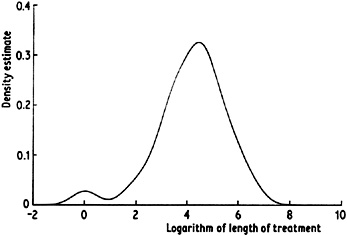
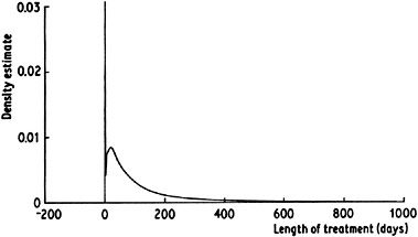
An example for which this treatment is clearly appropriate is the suicide data discussed earlier. Figure 2.12 gives a kernel estimate of the density underlying the logarithms of the data values; the corresponding density estimate for the raw data is given in Fig. 2.13. The relative undersmoothing near the origin is made abundantly clear by the large spike in the estimate.

Fig. 2.12 ernel estimate for logarithms of suicide study data, window width 0.5.

Fig. 2.13 Log-normal weight function estimate for suicide study data, obtained by transformation of Fig. 2.12. Note that the vertical scale differs from that used in previous figures for this data set.