


The redshifts of galaxies in the IRAS sample are affected by the same peculiar velocities that we are attempting to measure in the Mark III data set. If we measure redshifts cz in the rest frame of the Local Group, then
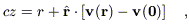
| (A1) |
where v(0)
is the peculiar velocity of the Local Group
and v(r) is the peculiar velocity at position r.
Indeed, because the galaxy density field shows coherence, the galaxy
density field measured in redshift
space  g(s)
differs systematically from that in real space,
g(r), as
was first described in detail by
Kaiser (1987;
cf. SW
and Strauss 1996
for reviews). The linear perturbation
theory assuming gravitational instability enables us to correct for the
effects of these velocities. We use here the iteration technique described
by Yahil et al. (1991)
and Strauss et
al. (1992c),
as updated by
Sigad et al. (1997).
The density and velocity fields are calculated within a sphere of radius
12,800 km s-1; the density fluctuation field is assumed to be
zero beyond this radius. Here we very briefly reiterate the
improvements described in the Sigad et al. paper and emphasize certain
differences from the approach there.
g(s)
differs systematically from that in real space,
g(r), as
was first described in detail by
Kaiser (1987;
cf. SW
and Strauss 1996
for reviews). The linear perturbation
theory assuming gravitational instability enables us to correct for the
effects of these velocities. We use here the iteration technique described
by Yahil et al. (1991)
and Strauss et
al. (1992c),
as updated by
Sigad et al. (1997).
The density and velocity fields are calculated within a sphere of radius
12,800 km s-1; the density fluctuation field is assumed to be
zero beyond this radius. Here we very briefly reiterate the
improvements described in the Sigad et al. paper and emphasize certain
differences from the approach there.
In regions in which the IRAS velocity field model predicts a nonmonotonic relation between redshift and distance along a given line of sight, it becomes ambiguous as to how to assign a distance to a galaxy given its redshift (Fig. 1). Our approach is similar to that used throughout this paper: we use our assumed density and velocity fields to calculate a probability distribution of a galaxy along a given line of sight.
Along a given line of sight, we ask for the joint probability distribution of observing a galaxy along a given line of sight, with redshift cz, flux density f, and (unknown) distance r:

| (A2) |
(cf. eq. [5]). The first term is given by our velocity field model along
the line of sight and thus is given by equation (9). For the iteration
code, we set  v
= 150 km s-1, independent of position, similar to the best-fit
value we find when we fitted for
v
from the velocity field data.
v
= 150 km s-1, independent of position, similar to the best-fit
value we find when we fitted for
v
from the velocity field data.
The second term is given by the luminosity function of galaxies:
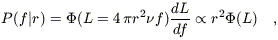
| (A3) |
where the derivative is needed because the probability density is defined in terms of f, not L. (16) Finally, the third term in equation (A2) is given by the galaxy density distribution along the line of sight (eq. [8]).
As described in Sigad et al. (1997), the calculations of the velocity and density fields are done on a Cartesian grid. Our approach therefore is to assign each galaxy to the grid via cloud-in-cell (weighting by the selection function, of course), where (unlike Sigad et al. 1997) we distribute each galaxy along the line of sight according to the distribution function of expected distance (eq. [A2]). In order to calculate the selection function for an object, we of course need to have a definite position for it; for this purpose, we assign it the expectation value of its distance, following Sigad et al. (1997):
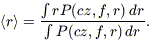
| (A4) |
Sigad et al. (1997) discuss the use of various filtering techniques to suppress the shot noise in the derived density and velocity fields. While they argue for the use of a power-preserving filter for the comparison of the IRAS and POTENT density fields, we have found through extensive experimentation with mock catalogs that for the VELMOD analysis, a Wiener filter gives the best comparison between the density field and the peculiar velocity data.
Finally, we found that when the iteration
technique was run to values
of 
 1, the
density field became unstable in the regions around triple-valued zones,
oscillating between iterations. We were able to suppress these by averaging
the derived density field at each iteration with that of the iteration
preceding it. This has no strong effect on the derived density field for
< 1.
1, the
density field became unstable in the regions around triple-valued zones,
oscillating between iterations. We were able to suppress these by averaging
the derived density field at each iteration with that of the iteration
preceding it. This has no strong effect on the derived density field for
< 1.
16 Eq. (144) of SW mistakenly left off this last term. Back.