Annu. Rev. Astron. Astrophys. 1980. 18: 489-535 Copyright © 1980 by Annual Reviews. All rights reserved

2. MEASUREMENTS OF THE SPECTRUM

Absolute measurements are always difficult. Measurements of the cosmic background radiation (CBR) spectrum are no exception and are further complicated by the fact that it is impossible to modulate the signal, the CBR. The CBR is therefore the residue, what is left over after one has accounted for everything else. The quality of this accounting, the precision and reliability of measurement of the individual terms, determines the value of the observation. The evolution of experiments to measure the CBR spectrum demonstrates this well. Future progress lies in unproved experimental design or operation. in more benign environments which permit reduction of the most uncertain elements in the accounting sum.

Direct measurements of the CBR spectrum fall crudely into two categories: low frequency observations in the Rayleigh-Jeans portion of the spectrum and observations at high frequencies in the region embracing the blackbody peak and into the Wien tail. This categorization results from the different technologies used in the two regions, and differences between the magnitudes of the terrestrial atmospheric emission. The low frequency measurements employ conventional microwave technology - coherent receivers - at sea-level and mountain observing sites while the high frequency observations have been carried out with less well developed infrared techniques - incoherent detectors, broad-band filters, Fourier transform spectrometers - on balloon- and rocket-borne platforms.

As the sub-millimeter technology of coherent receivers, in particular the development of efficient broad-band mixers, improves, the low frequency techniques will be applied to the high frequency region from balloon and aircraft platforms.

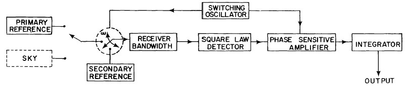
Figure 1 outlines the basis of all the low frequency measurements. The individual experiments listed in Table 1 may differ in details, even in some important ones, but nevertheless all consist of the same components: a coherent receiver, a primary absolute reference calibrator, and an antenna The experimental strategy has been to compare the radiation entering the antenna with that of the primary calibrator, the gain of the receiver being determined by either varying the temperature of the primary reference or by injecting a known power into the receiver input.

Figure 1. Schematic diagram of a generic absolute radiometer.

Table 1. Heterodyne measurements of the cosmic background spectrum

								Properties of primary calibrator
					Receiver	Beam	Thermodynamic	Antenna
		f	v	Altitude	noise	width	temperature of	temperature of	p Tp		w Tw
Reference	(cm)	(GHz)	(cm-1)	(km)	(K/Hz1/2)	(deg.)	primary ref	primary ref.	(K)	R	(K)
Howell &	73.5	0.41	0.014					1.7±0.2
Shakeshaft 1967				0	-	15	4.2	4.19		-	-
	49.2	0.61	0.020						1.4±0.2
Penzias &	21.2	1.415	0.047	0	-	-	4.2	4.17	0.6	-	-
Wilson 1967
Howell &	20.7	1.41	0.048	0	-	13×15	4.2	4.17	1.7±0.2	-	-
Shakeshaft 1966
Penzias &	7.35	4.08	0.136	0	-	-	4.2	4.10	1.3	-	-
Wilson 1965,
Penzias 1968
Roll &	3.2	9.37	0.313	0	-	20	4.2	3.98	2.6±0.35	-	-
Wilkinson 1966
Stokes et al. 1967	3.2	9.37	0.313	3.8	~ 1.5	4	3.77	3.55	0.16±0.10	6±3×10-4	0.06±0.02
Stokes et al. 1967	1.58	19.0	0.633	3.8	~ 1.5	4	3.77	3.33	0.21±0.08	1±0.3×10-3	0.04±0.01
Welch et al. 1967	1.5	20.0	0.666	3.8	~ 2	12	73.6	73.12	0.42±0.1	< 4.10-4	-
Ewing et al. 1967	0.924	32.5	1.08	3.8	~ 3	20	3.78	3.056	1.0±0.15	-	0.06±0.02
Wilkinson 1967	0.856	35.05	1.168	3.8	~ 1.5	4	3.77	2.99	0.28±0.11	0± + 3×10-4	0.06±0.06
Puzanov et al. 1968	0.82	36.6	1.22	0	1.6	4	77.36	76.48	-	-	-
Kislyakov et al. 1971	0.358	83.8	2.79	3	2-4	10	~ 75.0	~ 73.0	-	-	-
Boynton et al. 1968	0.33	90.0	3.00	3.44	1.5	-	3.8	2.042	0.22±0.11	3×10-4	0.27±0.04
Millea et al. 1971				3.1			3.85	2.087
	0.33	90.4	3.00		0.5	6.6			1.1±0.11	3±0.6×10-4	-
				2.8			3.88	2.114
Boynton &	0.33	90.0	3.00	14.9	0.1	-	4.2	2.405	0.22±0.11	8±4×10-4	0.27±0.04
Stokes 1974

Table 1. - continued

	Properties of antenna		External sourcesa
						Cosmic background
	ant Tant	fgnd Tgnd	atm Tatm	Tgal	Switch	thermodynamic
Reference	(K)	(K)	(K)	(K)	asymmetry	temperature	See note b
	0.4±0.2	0.6±0.4	1.3±0.1	20.6±2.2
Howell & Shakeshaft 1967					-	3.7±1.2	1,2
	0.4±0.2	0.6±0.4	1.95±0.1	6.7±0.7
Penzias & Wilson 1967	0.55		2.3	0.3	0.05	3.2±1.0	-
Howell & Shakeshaft 1966	1.3±0.2	0.1	2.2±0.2	0.5±0.2	-	2.8±0.6	2
Penzias & Wilson 1965,	0.8±0.4	0.1	2.3±0.3	< 0.2	0.05	3.3±1.0	3
Penzias 1968
Roll & Wilkinson 1966	1.08±0.15	-	3.0±0.2	< 0.0015	3.8±0.2	3.0±0.5	-
Stokes et al. 1967	0.08±0.06	< 0.05	1.37±0.1	-	-	2.69-0.21+0.16	4
Stokes et al. 1967	0.15±0.05	< 0.15	4±0.1	-	-	2.78-0.17+0.12	4
Welch et al. 1967	1.9±0.2	0.1	4±0.2	-	-	2.45±1.0	5
Ewing et al. 1967	0.2±0.06	0.03±0.01	4.6±0.2	-	0.5±0.1	3.09±0.26	6
Wilkinson 1967	0.12±0.04	< 0.05	6.5±0.2	-	-	2.56-0.22+0.17	4
Puzanov et al. 1968	-	-	17.0	-	-	3.7±1.0	5
Kislyakov et al. 1971	5±0.4	-	14.7±1.2	-	-	2.4±0.7	-
Boynton et al. 1968	0.21±0.12	-	11.5±0.22	-	-	2.46-0.44+0.40	4
Millea et al. 1971			11.8±0.22
	0.21±0.11	0.02		-	-	2.61±0.25	-
			12.1±~0.4
Boynton & Stokes 1974	-	-	1.21±0.37	-	-	2.48-0.54+0.50	7
						<T> = 2.74±0.087 K
						normalized 2 = 0.44
						14 degrees of freedom
FOOTNOTES FOR TABLE 1
a Atmospheric radiation entries are typical numbers for a data set. bNotes: The data analysis assumed that the cosmic background has a Rayleigh-Jeans spectrum and that the galactic component can be characterized by a power law spectrum. The two points together produce one measurement of the background temperature and the magnitude of the galactic emission. Atmospheric contribution is calculated from other data, not measured in the course of the experiment. Penzias & Wilson (1965) is the discovery observation. Penzias (1968) gives a corrected value for the measured temperature. The four Princeton experiments, due to their small error bars, have the largest weight in determining the average temperature. Looking at the data from the four experiments together, one can see that the measured contribution of the emission by the reflector scales only marginally with the square root of the frequency. The emissivity of idealized metal surfaces in the case Erf to the plane of incidence varies as ~ 2 cos ( / )1/2 where is the angle of incidence, the rf frequency, and the conductivity (cgs units). An aluminium reflector at 290 K has a minimum theoretical emission of 0.09, 0.125, 0.170, 0.27 Kant at 3.2, 1.58, 0.856, and 0.33 cm for = 30°. The published result has been converted to thermodynamic temperature. The emission by the horn antenna in this experiment is the estimated difference between the radiative contributions of two similar horns, one pointed to the load, the other to the sky. The published result has been corrected for an error in the way atmospheric absorption enters the measurement of the background radiation. The only 3 mm experiment in which the atmospheric contribution is less than the cosmic background. The apparatus was not calibrated using a primary calibration source during the airborne measurements. It was calibrated before and after flight. The properties of the calibrator were not remeasured and assumed to be the same as in Boynton et al. (1968).