Annu. Rev. Astron. Astrophys. 1980. 18: 489-535 Copyright © 1980 by Annual Reviews. All rights reserved

(d) Atmospheric Emission and Absorption

The profound role of the atmosphere in the measurements of the CBR is demonstrated in Figure 2 which shows the average atmospheric emission at four altitudes - 0, 4, 14, 44 km - as well as the Planck spectra of 300, 3, and 2.7 K blackbodies for reference. The curves correspond to the emission observed from the ground on a good day or night (column density of 1 cm precipitable H₂O), a mountain site (2 mm), the typical altitude attained by available and instrumented jet aircraft (10µ), and balloons (0.05µ).

Figure 2. Zenith atmospheric emission at various altitudes drawn for an instrument with 0.04 cm-1 hwhm resolution. The parameters are: 0 km (H2O, 3.7 × 1022 mol/cm2, 300 K; O2, 5 × 1024, 300; O3, 9 × 1018, 220); 4.2 km (7 × 1021, 250; 3 × 1024, 250; 9 × 1018, 220); 14 km (3.8 × 1019, 215; 6.7 × 1023, 215; 8 × 1018, 215); and 44 km (2.7 × 1017, 260; 1 × 1023, 260; 1.7 × 1017, 260).

All of the emission lines cone from rotational or fine structure transitions in the ground electronic and vibrational states of these molecules. The O₂ lines arise from two mechanisms - a cluster of lines at 2 cm^-1 and a single one at 4 cm^-1 originate from magnetic dipole transitions associated with the reorientation of the electronic angular momentum (2 Bohr magnetons from the unpaired electron spins) relative to the molecular rotation. (J = ±1, K = 0). These lines have been extensively studied experimentally (Meeks & Lilley 1963, Liebe et al. 1977). The other lines, occurring in triplets spaced 2 cm^-1 apart at 14, 25, 37 ... cm^-1, are magnetic dipole rotational transitions (J = ± 1, K = ± 2) predicted by Tinkham & Strandberg (1955a, b) and discovered by Gebbie et al. (1969). These lines play an important role in the recent and most precise measurement of the background spectrum at high frequencies (Woody & Richards 1979) and will be discussed in more detail later.

H₂O and O₃ are both asymmetric rotors with complicated spectra. H₂O, owing to its large electric dipole moment and relatively small partition sure at atmospheric temperature, is responsible for the bulls of the atmospheric emissivity in the spectral region (Benedict 1976). The influential H₂O lines are well separated in frequency. O₃, on the other hand, has a multitude of weak lines, no less than 300 in the 1 to 20 cm^-1 band (Gora 1959). A much appreciated and used resource is the Air Force Cambridge Geophysical Laboratory compilation of atmospheric line parameters (McClatchey 1979, Rothman 1978), which is available on magnetic tape. The compilation gives the frequency, line strength, energy of the ground state, and pressure-broadening coefficient of all known atmospheric lines from the radio through optical region.

It is well worth reviewing the assumptions and outlining the steps involved in calculating the models for atmospheric emission and absorption that have been used in CBR observations [Goody (1964) is a useful reference]. The end result of the calculation is the absorption and emission integrated over the atmospheric column at each frequency. The input parameters of a complete model would include 1. the temperature and partial pressure of the constituents as a function of altitude, 2. the individual molecular line strengths as a function of temperature, 3. the line shapes at different pressures and temperatures. To be complete, the Zeeman effect in the earth's magnetic field should be considered, especially at high altitude where the lines are narrow. The Zeeman effect makes the atmospheric propagation anisotropic. The calculation is carried out layer by layer beginning at some maximum altitude above which the radiation is deemed negligible. Each layer contributes its radiation and absorbs some fraction of the radiation from the preceding layer. The integration is continued to the altitude of the observation.

The complete calculation would pose a substantial computing problem, especially in maintaining sufficient frequency resolution to resolve the narrow lines at high altitudes. More important, the calculation is not worth doing. because many of the input parameters are poorly known. Except possibly for O₂, the partial pressure of the constituents as a function of altitude is the most uncertain element. The actual temperature distribution with altitude at the time of the measurement would be the next important unknown. Furthermore, the line profiles do not conform in detail to simple theoretical models because the collisional line-broadening mechanisms depend on the colliding species and their kinetic energies. At present the only reliable way to determine the line-broadening parameters is to measure them directly with high resolution instruments.

All this is not to say the atmosphere is impossible to model but rather to urge caution in the interpretation of absolute CBR measurements where the atmospheric contribution is large.

In those parts of the atmospheric spectrum where the total absorption is small, less than ~ 10%, the atmospheric emission can be measured by zenith angle scanning, since the emission is linearly proportional to the total column density of emitters. The result depends only on the assumptions of a laminar atmosphere and homogeneity within each layer and not on the specific model. Temperature, pressure, and constituent inhomogeneities occur and in fact are the largest source of random noise in the ground-based experiments. However, they do not contribute systematic errors unless the particular observing site is anisotropic in a gross manner - because of a large lake or the ocean in the direction of the zenith scan, for example. 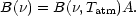The atmospheric and CBR contributions are separable in this case without further measurements or modeling. The total emittance B as a function of zenith angle is given by

(4)

where (f, ) is the atmospheric absorption coefficient (in this case also the emissivity) at frequency f which is proportional to the column density of emitters (absorbers) and therefore depends on sec. B(f, T) is the blackbody emittance at the thermodynamic temperature T. Measurement of B(f, ) at two angles gives B(f, T_CBR) to a theoretical precision of order ². The procedure implied by Equation (4) has been used in all of the low frequency ground-based measurements.

Since the atmosphere at low frequencies appears primarily as a random noise source rather than a systematic one, there is hope for improved measurements of the CBR at low frequencies from the ground, The strategy of using two frequencies, X (3 cm) and K band (1.5 cm), simultaneously with up-to-date low noise radiometers, would allow measurement of the atmospheric fluctuations during the course of zenith scanning. Furthermore, rapid zenith scanning with co-addition of scans would overcome some of the dominating low frequency components of the atmospheric fluctuations.

Once self-absorption becomes important, atmospheric modeling is inevitable; Equation (4) then looks more like

(5)

although this equation still does not represent the complete integration required.

The atmospheric absorption coefficient and the atmospheric blackbody emittance no longer appear as a simple product and must be calculated or determined separately as a function of altitude, h. Zenith scanning no longer gives a model-independent measure of the atmospheric contribution. The CBR observations at high frequency from balloons had to face up to this.

The multifilter MIT (Muehlner & Weiss 1973a, b) and the Berkeley spectrometer experiments (Woody et al. 1975, Woody 1975, Woody & Richards 1979) have used similar strategies to handle the atmospheric contribution. At high altitudes the individual molecular lines are narrower than the spectrometer or filter resolution widths. Pressure line-broadening parameters range around 0.1-0.3 cm^-1 per atmosphere pressure so that, at an altitude of 44 km (pressure 2 × 10^-3 atm), the line widths at the base of the column are ~ 10^-4 cm^-1. Doppler widths are typically a factor of 10 smaller (as a consequence, absorption of the CBR is neglected). The difference between Van Vleck-Weisskopf and Lorentzian line shapes becomes negligible for such narrow lines and the Lorentzian profile is adopted for ease of calculation. All the emitting constituents are assumed to be uniformly mixed with an exponentially decreasing density as a function of altitude. The emitting column is furthermore assumed to be isothermal with the temperature measured at its base.

Under these assumptions, the power in a line from the column, integrated over all frequencies, can be cast in an analytic form that depends on the total column density, the line strength, the pressure-broadening parameter, and the temperature (Goody 1964). The equivalent emission width of the line is given by

(6)

where x is a dimensionless parameter indicating the degree of saturation of the line given by

(7)

S(T) is the line strength in units of cm^-1 / molecule / cm² and includes the matrix elements, multiplicity, fraction of molecules in the lower state, and the relative population difference of the two levels involved in the transition. (T, P₀) is the pressure-broadened Lorentzian line width at the base of the column, and is the column density in molecules/cm². The total emittance due to the line is

(8)

The limiting cases are

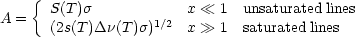When the lines are unsaturated (the emissivity at line center is much less than 1), the emission is linearly proportional to the column density and therefore the atmospheric contribution could be measured directly with zenith scanning in an almost model-independent determination. On the other hand, if the line is saturated, the emission is proportional to the square root of the column density - this is due to the assumed Lorentzian line function - and depends on the pressure-broadened line width. The increase in emission with column density can only come from molecules emitting in the wings of the line. Zenith scanning would produce an atmospheric signal proportional to (sec)^1/2 and, providing that all lines falling into the instrument resolution width were saturated, could be used to aid in determining the atmospheric contribution. The real problem comes with a mixture of both saturated and unsaturated lines or partially saturated lines, which is the situation in the stratospheres the O₂ fines are partially saturated, the strong H₂O lines are fully saturated, and all O₃ lines are unsaturated. Zenith scanning, with an instrument of low frequency resolution, can without knowledge of the individual constituent column densities only offer a model-independent lower limit to the atmospheric radiation and hence an upper limit to the CBR. This was the case with the MIT experiments (Muehlner & Weiss 1973a). A subsequent flight by this group (Muehlner & Weiss 1973b) used different narrow-band filters to isolate individual atmospheric lines of H₂O and a cluster of O₃ lines to determine the constituent column densities, but the signal to noise and flight duration were insufficient to improve substantially on their prior results. The spectrometer observations have enough resolution to isolate the lines of O₂ and H₂O and line clusters of O₃ so that it becomes possible, using the model outlines above, to solve for the individual column densities by fitting the observed spectrum.

A question that beeps recurring when the high frequency balloon measurements are discussed is the validity of the simple atmospheric model, which is inadequate at lower altitudes. In preparing this review I made a comparison over a restricted frequency band (10-20 cm^-1) of the model described above at 43 km with a 10 layered one that 1. used Doppler lines in the upper stratosphere and Van Vleck-Weisskopf lines at lower altitudes, 2. removed the isothermal restriction using the average atmospheric temperature profile with altitude (US 1966), 3. retained the uniform, mixing hypothesis. The same line parameters were used in both calculations but the estimated temperature dependences of both the line strengths and line-broadening parameters were included. The result was that for the same column base temperature and pressure and equal column densities, the two models differed by less than 5%, not a remarkable result since the major emission occurs within a scale height. The difference between models is no worse than the "noise" of the uncertainties in the line parameter listings, which I estimate to be at least 10%.

Another recurring worry is the possibility that there exist influential atmospheric constituents that emit in this spectral region but are not now included in the line listings. The response is an equivocal "no." Finally, the notion of calibrating a CBR experiment using the atmospheric emission is a bad one; more on this later.