Copyright © 1980 by Annual Reviews. All rights reserved
| Annu. Rev. Astron. Astrophys. 1980. 18:
489-535 Copyright © 1980 by Annual Reviews. All rights reserved |


(g) High Frequency Observations of the Spectrum
The high frequency experiments have gone through two generations. The first were the rocket- and balloon-borne observations using cryogenic broad-bared radiometers which laid the technological groundwork for the second and present generation of high resolution cryogenic spectrometer observations. Some of the broad-band experiments were discussed in the Thaddeus (1972) review and the final results of these observations are listed in Table 2. The earliest experiments in the late 1960s were attended by controversy; the first rocket observations of the Cornell group showed a large energy excess at high frequencies, while the first multifilter radiometer balloon experiments of the MIT group shoved an excess in one of three spectral channels. By the early 1970s the rocket experiments, in particular those of the Los Alamos group and a new set of balloon observations of the MIT group using 5 spectral channels, settled the controversy. Furthermore, with the improved understanding of the atmospheric emission by 1973, the balloon experiments had established that there was a peak in the CBR spectrum and that the total power was consistent with the extrapolation of the ground-based low frequency measurements. The detailed shape of the spectrum was, however, not measured.
| Beam | P(side lobe+warm parts) | P(atmosphere) | ||||
| Band | Altitude | size | CBR | |||
| Reference | (cm-1) | (km) | (deg.) | P(total) | P(total) | (K thermodynamic) |
| Houck et al. 1972 | 7.7-25 | 144 | ~ 2 | ? | - |  4.1 4.1 |
| Williamson et al. 1973 | 1.7-12.5 | - | 3.4-3.4+1.4 | |||
| 1.7-16.7 | 325 | 20 | ? | - | 5.1-1.5+0.8 | |
| 1.7-33.3 | - | 3.8-1.9+0.8 | ||||
| Muehlner & Weiss 1973a,b | 1-5.4 | 44,39 | 10 | < 0.04 | 0.13 | 2.7-0.6+0.4 |
| 1-7.8 | < 0.04 | 0.09 | 2.8±0.2 | |||
| 1-11.1 | < 0.05 |  0.53 0.53 |
2.7 |
|||
| 1-18.5 | < 0.02 | 0.73 |
3.4 |
|||
| Dall'oglio et al. 1976 | 7.1-11.1 | 3.5 | 2 | ? | 0.8 |
2.7 |
Some of the underlying problems in the early experiments are still manifested in the second generation experiments. The worst and unavoidable problem is just the fact that a fussy absolute observation must be carried out by remote control; the effect of this is that in the course of the experiment what might have been an easy calibration or test for a systematic error, or iteration in the experiment design, turns into a substantial and often expensive engineering project. The next order difficulty is due to interaction of three factors: small observation times, inadequate test facilities, and low sensitivity detectors. The nonthermal equilibrium environment - a 3 K sky, a hot earth below, and in the case of a balloon experiment, a warm and condensable atmosphere surrounding the apparatus - are difficult to simulate in terrestrial test facilities. As a consequence the final testing for systematic errors and in principle the calibration under the actual observing conditions must (or should) be carried out during the course of the experiment. The total observing time in a rocket observation is measured in minutes while for balloons it is approximately 10 hours. At very high altitudes where the atmospheric emission is smallest, the stratospheric winds are irregular and strong and the observing tinges may only be a few hours. With time so limited, a premium is put on having sensitive detectors to test for systematic error sources such as the contribution from warm parts of the surroundings and side-lobe response, to mention just two. The detectors have unproved considerably. In the early experiments the detector noise equivalent power (NEP) was ~ 10-11 to 10-12 W/Hz1/2, just barely good enough to measure the total power in the CBR in seconds of integration time with systems of 10% optical efficiency and an étendue of 0.1-0.3 cm2 sr. Present day detectors (composite bolometers) are a factor of 100 to 1000 more sensitive and the second generation experiments have made good use of them. But the fact remains that a table, such as Table 1, developed for the love frequency experiments, cannot assembled for the high frequency experiments under observing conditions, and further, none of the high frequency experiments have experienced a primary calibration during flight.
All the high frequency spectroscopic observations of the CBR have employed Fourier transform spectrometers - Michelson interferometers. In these devices the incident radiation is split between two paths and recombined after one path is delayed relative to the other. The output signal as a function of the delay is the autocorrelation function of the radiation which, Fourier-transformed, becomes the power spectrum.
Fourier transform spectrometers are the logical choice for measuring the small power in the CBR with present day detector technology since they offer a wide spectral range, typically 2 decades, multiplexed on one or two detectors, and a large étendue, 0.1 to 0.5 cm2 sr. The optical efficiency of the spectrometer in the millimeter and sub-millimeter range cars approach 100% by using polarizing Michelson interferometers (Martin & Puplett 1969) in which the beam division is performed by a polarizer, an almost ideal optical component at these wavelengths. The frequency resolution is adjustable and limited by the maximum delay for which beam divergence or wave front distortion and displacement within the instrument destroys the relative spatial coherence of the two recombined paths. Resolutions of a few tenths of a wavenumber are typical for the instruments that have been used.
Fourier transform spectroscopy is not without hazards, the most serious being the opportunities for frequency distortion of the measured spectrum. Total intensity variations due either to fluctuations in the input signal (random noise) or incurred by the scanning (systematic errors), transform into spurious frequency components in the spectrum. Systematic spectrum. distortions can also result from periodic errors in the mechanism that produces the delay. Careful design reduces these errors and thorough calibration can uncover them. A safe way to reduce their effect is to limit the optical bandwidth of the system but this of course limits the spectral coverage. The high optical efficiency, étendue, and multiplexed frequency coverage also put burdens on the detector linearity. Consequently calibration of the spectrometer requires care so as not to saturate the detector and is best carried out with cryogenic thermal sources. The emittance measurable with a Fourier transform spectrometer is given qualitatively by
 |
(14) |
where T( ),
A
),
A , and
, and
 opt are
the overall optical transfer function, étendue,
and optical efficiency of the system t is the total observing time
using a detector with a given NEP to achieve a signal to noise S/N, in
estimating the emittance in a frequency resolution element
opt are
the overall optical transfer function, étendue,
and optical efficiency of the system t is the total observing time
using a detector with a given NEP to achieve a signal to noise S/N, in
estimating the emittance in a frequency resolution element
 res.
B0() is the
thermal radiation by the interferometer enclosure or an absorbing
surface entering the other port of the interferometer or incident on the
detector during the
alternate half of the chopping cycle when the instrument "looks" at itself.
The contribution from this term produces an offset which, if constant
throughout the measurement, can be determined from the external absolute
calibration.
res.
B0() is the
thermal radiation by the interferometer enclosure or an absorbing
surface entering the other port of the interferometer or incident on the
detector during the
alternate half of the chopping cycle when the instrument "looks" at itself.
The contribution from this term produces an offset which, if constant
throughout the measurement, can be determined from the external absolute
calibration.
The design of the three high frequency spectroscopic instruments used in
CBR measurements are shown in Figures 4,
5, and 6. The Queen Mary
College balloon-borne instrument
(Beckman & Robson 1972,
Beckman et al. 1974,
Robson et al. 1974),
Figure 4, is a cryogenic polarizing Michelson
interferometer operated at 1.4 at 40 km altitude. The instrument
parameters are 0.1 cm2 sr étendue, 0.25 cm-1 unapodized
resolution, 6°
beam width maintained at a 50° zenith angle during flight. The
beam was defined by the 45° off axis paraboloid collimator at the
entrance of the
interferometer section after the beam had traversed a warm 50µ
polyethlyne window (not shown in the figure) and a stationary entrance
polarizer followed by a rotating polarizer used as a chopper. Two InSb
hot electron bolometers detect the beans reflected and transmitted by
the output polarizer yielding two interferograms 180° out of
phase. The technique of
chopping with a rotating polarizer eliminates the signal that is not
modulated by the delay and thereby reduces one opportunity for frequency
distortion of the spectrum. The overall system transfer function has not
been published but must be dominated by the high frequency roll off of the
InSb detectors beginning near 10 cm-1 varying as
1 / and then
further attenuated above 40 cm-1 by the reduced efficiency of the
polarizers as the wavelength approaches the polarizer grid spacing
(100µ).
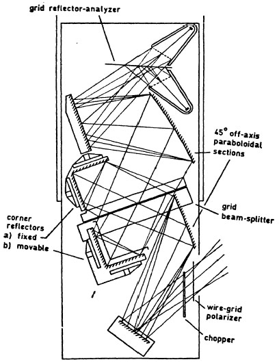 |
Figure 4. The Queen Mary College polarizing Michelson Interferometer. |
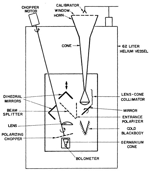 |
Figure 5. The Berkeley polarizing Michelson Interferometer. |
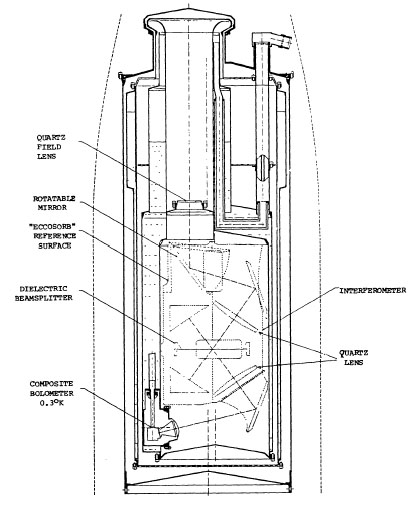 |
Figure 6. The rocket-borne Michelson interferometer of Gush. |
I have difficulty in evaluating the results of the experiment, Figure 7, as there are inconsistencies in the data and the accounting of the radiation incident on the instrument is incomplete. The emission by the warm polyethlyne window, which. is not removed during the observation, is unknown and may never be known as it is possible that frost condensed on it. An estimate of the atmosphere emission has not been published. However, an attempt (on my part) to model the atmosphere as observed in this experiment, especially in the critical minimum. between 8 and 18 cm-1, fails by a substantial margin. The contribution of the ground in the beam side lobes due to diffraction by edges at the entrance optics has not been published; finally, the calibration of the instrument in flight is not established.
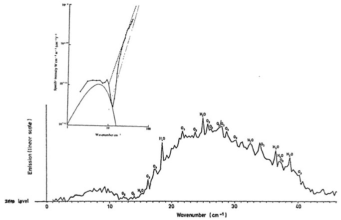 |
Figure 7. Spectra of the sky derived from the Queen Mary College instrument. The lower trace is the total measured spectrum including the CBR, an unknown window emission, and the atmosphere at 40 km (50° zenith angle) uncorrected for the instrument transfer function and without an absolute vertical scale. The unapodized resolution of the spectrum is 0.25 cm-1. The insert is the corrected spectrum including several estimates of the window emission. The solid line is the difference between a 2.7 K and a 1.4 K spectrum. |
The Berkeley balloon-borne experiment, Figure 5
(Mather 1974,
Mather et al. 1974,
Woody 1975,
Woody et al. 1975,
Woody and Richards 1979),
has been flown twice successfully with improvements in the apparatus between
flights. The instrument is again a polarizing Michelson using germanium
bolometers. A composite bolometer maintained at 0.3 K (NEP
1 × 10-15
W/Hz1/2 was used in the second flight, which enhanced the
sensitivity of the instrument by a factor of 10. The instrument
parameters are 0.23 cm2 sr 6tendue, maximum unapodized
resolution 0.14 cm-1, 6° beam width, and
an overall optical efficiency in mid-band ~ 1%. A. significant
feature of the
design is the beam-forming cone, held at liquid helium temperature, which
has a demonstrated and calculable o axis rejection of 106 at
60° and
greater for larger angles. In the second flight an even better cone was
used in
concert with ground shields. Zenith scanning measurements carried out
during flight demonstrated that the large angle contributions from the
earth were less than 5 × 10-13
1/2 W/cm2 sr
cm-1. In flight, the window over the
cone was removed. The primary calibration was carried out on the ground
with cryogenic calibration sources placed in the beam-forming cone.
Calibration in flight, however, was estimated with an ambient temperature
secondary calibrator that could be swung into the beam. The cold
blackbody source inside the interferometer at the temperature of the
interferometer enclosure served to establish the offset.
The data of the second flight, Figure 8, are the most precise measurements of the CBR spectrum to date at high frequencies. (The data of the first flight is much the same with decreased signal to noise.) Panel a is the instrument transfer function which has been rolled off at high frequencies by a low pass filter at the detector. Panel b is the total measured spectrum uncorrected for the instrument transfer function while c is the fitted atmospheric emission spectrum using the techniques described previously. The scheme used by the group was to fit the interferogram rather than the spectrum to the atmospheric model. This streamlines the computations, eliminating the need to calculate the convolution of the instrument response function with the fitted spectrum. Panels d and e are the residuum, in principle the CBR at 0.28 and 1.8 cm-1 resolution. The data corrected for the instrument transfer function are given in numerical form in Table 3 (D. P. Woody, 1979, private communication).
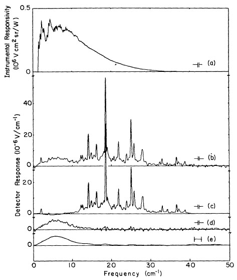 |
Figure 8. The Berkeley spectrum. Panel a shows the instrument transfer function. Panel b shows the total measured spectrum uncorrected for the instrument transfer function. The spectra are derived from asymmetric interferograms of 3.72 and 0.48 cm optical delay on either side of the central maximum. The apodization used is (1 - x2 / L2)2. The resolution of the larger optical delay is 0.28 cm-1 but with wings from the shorter delay. Panel c is the best fit of b to the model atmosphere and instrument offset. Panel d shows the residual and e the same residual with 1.8 cm-1 resolution. The lines at 12,14, and 16 cm-1 are a group of the O2 pure rotational lines discussed in the text. |
The Berkeley data deserves close scrutiny because the major terms in the
accounting are measured. Treating the errors in flux determination at each
frequency as independent, the best fit to a. Planck spectrum, with
temperature as the only fitted parameter, is TCBR =
2.96 K at
only a 35%  2
contour - a 1 in 3 chance that data with the assumed random errors would
fit as poorly as it does if the true spectrum were thermal at this
temperature. In other words, the deviations from a thermal spectrum at
2.96 are statistically significant. The question is, are these
deviations real or artifacts
of observation? Caution driven by experience dictates that we be hard on
the experiment. The weakest link in all the high frequency CBR spectrum.
experiments is in the absolute calibration, not so much in the spectral
response of the instrument but rather in the overall frequency-independent
scale factor that converts the measured signal into an absolute power
incident on the instrument.
2
contour - a 1 in 3 chance that data with the assumed random errors would
fit as poorly as it does if the true spectrum were thermal at this
temperature. In other words, the deviations from a thermal spectrum at
2.96 are statistically significant. The question is, are these
deviations real or artifacts
of observation? Caution driven by experience dictates that we be hard on
the experiment. The weakest link in all the high frequency CBR spectrum.
experiments is in the absolute calibration, not so much in the spectral
response of the instrument but rather in the overall frequency-independent
scale factor that converts the measured signal into an absolute power
incident on the instrument.
1
 flux limits flux limits |
1
TCBR
limits (K) |
||||
| v | Average flux | ||||
| (cm-1) | (10-12w/cm2 sr cm-1) | min. | max. | min. | max. |
| 2.38 | 8.74 | 7.76 | 9.99 | 3.05 | 3.57 |
| 3.40 | 12.13 | 11.02 | 13.67 | 2.95 | 3.29 |
| 4.41 | 14.81 | 13.65 | 16.51 | 2.97 | 3.22 |
| 5.42 | 16.05 | 14.81 | 17.89 | 2.97 | 3.18 |
| 6.44 | 16.09 | 14.86 | 17.94 | 2.98 | 3.16 |
| 7.45 | 13.89 | 12.76 | 15.57 | 2.91 | 3.07 |
| 8.46 | 12.42 | 11.36 | 13.98 | 2.92 | 3.07 |
| 9.48 | 8.63 | 7.71 | 9.89 | 2.79 | 2.94 |
| 10.49 | 6.64 | 5.21 | 7.75 | 2.76 | 2.91 |
| 11.50 | 5.52 | 4.48 | 6.74 | 2.75 | 2.95 |
| 12.52 | 4.07 | 2.69 | 5.47 | 2.66 | 2.97 |
| 13.53 | 4.92 | 2.82 | 7.15 | 2.80 | 3.23 |
| 15.20 | 1.87 | - | 4.10 | - | 3.15 |
| 17.28 | 0.96 | - | 3.07 | - | 3.27 |
| 20.03 | 0.70 | - | 1.81 | - | 3.36 |
| 22.89 | 0.48 | - | 5.76 | - | 4.21 |
In the Berkeley experiment, primary calibration before and after flight
agreed but the instrument was not directly calibrated with the same
precision during flight, the properties of the secondary ambient
temperature calibrator not being well enough known. If one then assumes
(without specific justification) that the instrument behaved differently
in flight, one might try a two-parameter fit to the data, fitting to a
thermal spectrum and a frequency-independent overall calibration
factor. The results of this
procedure are T = 2.79 and a calibration factor of 1.27. The
2
contour is close to 90%, a very good fit.
Woody & Richards (1979)
point out this fact
and argue that a 27% calibration error is inconsistent with the emission
measured by the atmospheric O2 lines. The argument hinges on
the fact that emission by O2 is the one atmospheric
contribution that can be calculated directly. The calculation is built
on the following assumptions: 1. the O2 column density
(uniformly mixed) is given by
the barometric pressure at altitude, 2. the column temperature
distribution is known, 3. the line shapes
are known, and finally 4. the tabulated line parameters are correct.
In preparing this review I redid the O2 calculations
independently and agree with the Woody & Richards result using the
current best theoretical
estimates of the line strengths and line widths of the magnetic dipole
rotational transitions
(K = ± 2)
(Greenebaum 1975,
Liebe et al. 1977,
Weiss 1980).
However, there is little direct experimental evidence of the line
strengths, and in particular the pressure widths, except for
measurements of insufficient absolute precision by
Debbie et al. (1969),
which incidentally
give smaller line strength than the theoretical values. Furthermore, the
Zeeman effect of O2 in the earth's magnetic field must be
treated in detail and this is still in progress. The O2 fine
structure line,
K = 0, at 4
cm-1 is
far better known and would serve as a more reliable calibration but the
instrument transfer function is changing rapidly at this frequency. The
conclusion is that there are too many uncertainties in the calculation to
allow an absolute calibration to a precision of 30% using the atmospheric
emission.
The rocket-borne instrument of Gush (1979), Figure 6, performed the first spectrometer observations of the CBR above the atmosphere. The observations took place in the approximately 7 minutes while the payload was between 370 and 150 km altitude. The instrument is a conventional but cryogenically cooled Michelson interferometer using a dielectric pellicle beam splitter and a composite bolometer operated at 0.3 K. The interferogram is developed by varying the delay at a constant rate without additional beam chopping (rapid scan mode of operation). The instrument transfer function is determined by the reflection spectrum of the beam splitter at long wavelengths, becoming more inefficient the longer the wavelength, and by both the beam splitter and the high audio frequency roll-off of the detector and associated electronics at short wavelengths. The optical bandwidth of the interferometrically unmodulated component of the input signal is large, extending past 35 cm-1, and this may have aggravated one of the difficulties experienced in the experiment. The instrument was calibrated before and after flight with a cryogenic reference source.
Unfortunately the results of the experiment, Figure 9, are tentative because the analysis of the data requires modeling of a significant time-varying radiative contribution from the rocket clam shell covers that moved unexpectedly to the edges of the spectrometer beam. Another time-varying and significant correction had to be made for the temperature variation of the entire instrument due to venting of helium efflux gas during the course of the flight.
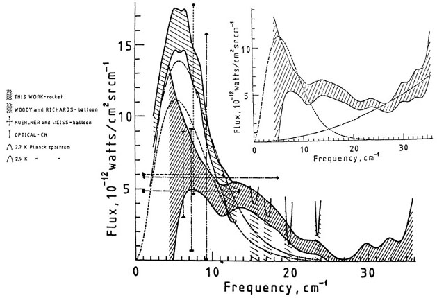 |
Figure 9. Rocket data of Gush. The inset shows the measured spectrum corrected for the instrument transfer function. The spectrum includes a contribution from hot objects at the edges of the beam modeled by the dot-dash line. The larger figure is a composite of various measurements of the CBR spectrum at high frequency. |
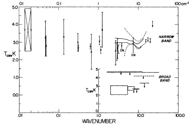 |
Figure 10. Summary of the measurements of the thermodynamic temperature of the CBR as a function of frequency. |
Figure 10 summarizes the direct measurements of the CBR spectrum and includes the determinations using the excitation temperature of CN observed in molecular clouds at 3.79 and 7.58 cm-1 (Thaddeus 1972, Hegyi et al. 1974, Danese & DeZotti 1977). The figure gives the thermodynamic temperature of a blackbody source with the same flux as that measured. The uncertainty in flux is related to the uncertainty in temperature by
 |
(15) |
In summary, the overall shape of the spectrum is thermal, characterized by a single parameter, the temperature. Considering the moderate precision of the low frequency experiments and the uncertainties in the high frequency observations, it is, in my opinion, too early to fruitfully analyze the present data for the subtle distortions that may discriminate different cosmic histories. Another generation of observations is needed.
CBR measurements using optical spectroscopy to probe the state of excitation of interstellar molecules equilibrated to the background radiation have not advanced since 1974. It would be delightful to observe the CBR at different locations in the universe and at different times by in situ measurements using molecules in other galaxies. The idea may be fanciful but not entirely impossible.