Annu. Rev. Astron. Astrophys. 1980. 18: 489-535 Copyright © 1980 by Annual Reviews. All rights reserved

3. MEASUREMENTS OF THE LARGE ANGULAR SCALE INTENSITY DISTRIBUTION OF THE CBR

The most convincing evidence that the background radiation is of cosmological origin - due to very distant sources if not the primeval explosion - is its isotropy, or more explicitly, that it does not share the anisotropy distribution associated with local sources such as the solar system or the Galaxy. The CBR, in fact, exhibits such a high degree of isotropy on both small (< 1°) and lane angular scales, short of the dipole term, as to pose a quandary. On small angular scales, no evidence has yet been found for granularity, thereby stringent limits are set on any discrete source hypothesis for the origin of the background. On the other hard, at some level, still not observed, small scale anisotropies must occur as density perturbations in the early universe are believed to have preceded the presently observed aggregations. The status of these observations is not part of this review [see the article by Partridge in Ulfbeck (1980)]. On large angular scales ( 10°), the anisotropy of the CBR is less than 1/3000, limited only by measurement uncertainties, lending strong support to the naive assumptions of homogeneity and isotropy made in developing the spherically symmetric cosmological models, but leaving the puzzle of how unconnected regions of the universe could have evolved so identically.

In addition to the search for evidence of intrinsic cosmic anisotropies, such as night be due to aspheric expansion or large scale anisotropies in the primeval matter distribution, an impetus for the lame angular scale isotropy experiments has been the measurement of the kinematic anisotropy associated with the earth's motion relative to the distant sources of the CBR. This anisotropy had to exist at least on a level of 10^-4 due to the earth's orbital motion around the sun in the unlikely case that the sun were at rest with respect to these sources. The anisotropy, now definitely observed at a 10^-3 level is easily derived by a special relativistic calculation of the intensity measured by an observer moving relative to the walls of a blackbody cavity. The anisotropy retains a Planck spectrum but with an observation angle-dependent temperature (dipole term) given by

where T₀ is the temperature observed in a frame at rest with respect to the sources, v is the velocity of the observer, and is the angle between the observing direction and the velocity.

Kinematic anisotropies of higher order (quadrupole) could exist if the universe rotates (Collins & Hawking 1973) or is filled with long wavelength gravitational radiation (Burke 1975). In general, the intensity distribution expanded in spherical harmonics is a convenient method of interrelating observation and theory in. this almost spherically symmetric system. To date, no positive evidence exists for moments higher than the dipole; however, as the measurement sensitivity improves and, in particular, the sky coverage becomes more complete, interesting limits (if not measurements) can be set on the higher moments. Both extended sky and spectral coverage will become essential to unscramble the effect of local sources which are expected (Figure 3) to become important at 10^-4 anisotropy levels even in the clearest region of the CBR spectrum. The measured spectrum of the dipole anisotropy is close to thermal. If this holds for higher order anisotropies, it becomes a discriminant against the local sources with their own characteristic spectra. Sky coverage is also required to break the correlation in estimates of the amplitude of different multipole moments. Higher order moments, if they exist, corrupt estimates of the lower order moments in fitting the multipole expansion with a data set derived from partial sky coverage.

Isotropy experiments do not have the same character as those designed to measure the CBR spectrum. The major difference is, of course, that isotropy experiments make relative measurements. The quantity measured is the difference in intensity from different directions; absolute calibration, therefore, plays a secondary role. Furthermore, because one is looking at a fixed structure in the celestial sphere, the differential data can be tested for internal consistency. Apparatus- and environment-generated anisotropies can, in principle, be removed by observing the same celestial locations under different experimental conditions. In other words, the data alone, without farther accounting as in the spectrum observations, can reveal whether or not the experiment is in trouble. The ultimate systematic errors come from local astrophysical sources, in particular from extended objects or regions of low surface brightness which may have eluded less sensitive sky surveys.

Receiver or detector sensitivity is at a premium in these experiments because the CBR anisotropies are small and tests for systematic noise in the instruments have to be carried out at the same low levels. Present day receivers at 20-30 GHz have sensitivities (Equation 1) ~ 50 mK / Hz^1/2. Observation of a systematic effect at the 10^-3 anisotropy level requires ~ 10 minutes of integration time. In the near future, Maser preamplifiers will be used at 20 GHz, increasing the sensitivity by a factor of 10 to 20 (S. Gulkis and D. T. Wilkinson, private communication). Broadband mm and sub-mm incoherent radiometers using composite bolometers have achieved sensitivities ~ 1 mK / Hz^1/2 (2.7 K). However, at these high frequencies the galactic dust background (systematic errors) and the residual atmospheric fluctuations, even at balloon altitudes (random errors), intrude.

Table 4 presents the results and some of the characteristics of large scale anisotropy experiments. All experiments, except those of Penzias & Wilson (1965) and Wilson & Penzias (1967), who mated in their discovery paper that the background was isotropic to 10%, have been carried out by comparing the intensity from one part of the sky with that from another without reference to an absolute calibrator. The early ground-based experiments were plagued by the large galactic background at long wavelengths and atmospheric emission fluctuations at shorter wavelengths where the galactic background is smaller. In these experiments, the radiation from two directions at the same elevation angle (to equalize the average atmospheric contribution) is compared as the earth's rotation sweeps the beams over the sky. Various scanning strategies were used. Partridge & Wilkinson (1967) compared the radiation from the celestial equator with a fixed point at the celestial pole using a single beam switched by a large mirror. This experiment established that the CBR anisotropies were less than a few parts in a thousand. Conklin (1969, 1972) compared the radiation entering two horns set at 30° to the zenith (fixed declination 32°), one pointing toward the east, the other toward the west. The horns were periodically interchanged in order to search for systematic differences in the apparatus. This experiment was the first to report a 24 hour anisotropy but the result was tentative because the large galactic contribution had to be modeled by extrapolation with a poorly known spectral index from 400 MHz sky maps. The observation, which measured the East-West component of the anisotropy, agrees with newer measurements, but it took courage to publish the result at the time. Boughn et al. (1971) attempted an isotropy measurement at 35 GHz, where the galactic contribution is small. The instrument was a differential radiometer with one beam (the reference) pointed to the zenith and the other switched periodically between two points on the celestial equator 2.1 hr either side of the meridian plane. Atmospheric emission fluctuations dominated the noise budget, partly aggravated by the experiment design, but nevertheless highlighting one of the main difficulties with ground-based large angular scale anisotropy experiments. The sensitivity to a dipole anisotropy increases as the sine of the beam separation. However, the effect of atmospheric emission fluctuations grows as well, since the fluctuations become more independent the larger the beam separation.

Table 4. Results of large scale anisotropy experiments

					Receiver	Beam
		f	v	Altitude	noise	width	Trms mK	T mK
Reference	(cm)	(GHz)	(cm-1)	(km)	(mK / Hz1/2)	(deg.)	Beam width	(24 hr)
Wilson & Penzias 1967	7.35	4.08	0.14	0	-	-	< 100	-
Partridge & Wilkinson 1967	3.2	9.4	0.31	0	-	10	~ 10	1±2.2
Conklin 1969	3.75	8.0	0.27	3.8	65	12	-	1.6±0.8
								(projected
								= 32)
Conklin 1972								2.3±0.9
								equitorial
Boughn et al. 1971	0.86	35	1.16	0	1600	4	~ 50	7.5±11.6
Henry 1971	2.96	10.1	0.34	24	~ 250	15	3	3.2±0.8
Corey & Wilkinson 1976	1.58	19	0.63	25	100	~ 10	3	2.9±0.7
Corey 1978
Muehlner & Weiss (Muehlner 1977)			3-10	39	90	18	3	< 3.3
Smoot et al. 1977	0.9	33	1.11	20	44	7	1.5	3.5±0.6
Gorenstein 1978
Cheng et al. 1979	1.21	24.8	0.83	27	51	8	1.5
								2.99±0.34
	0.955	31.4	1.05	27	45	6	1.5
Analysis includes Corey 1978
Smoot & Lubin 1979	0.9	33	1.11	20	44	7	1	3.1±0.4
							(95% CF)
Muehlner & Weiss 1980	-	-	3-10	39	90	18	3	2.8±0.8
Note: Since this review was written the measurement of the large scale anisotropy in the 3-20 cm-1 band has been reported by Fabbri et al. (1980). The data imply a dipole anisotropy of amplitude TD = 2.9-0.6+1.3 mK in the direction D = 11 h 24 m ± 40 m, D = 3 ± 10°. The data require a fit to a quadrupole-like term of amplitude 0.9-0.2+0.4 mK.

Table 4 - continued

	T mK
	(24 hr
	galactic	RAD		T mK
Reference	correction)	(hr)	D	(12 hr)	Sky coverage
Wilson & Penzias 1967	-	-	-	-	29 Locations distributed
					70° > > - 20°
					2 hr < < 20 hr
Partridge & Wilkinson 1967	-	-	-	4.9±2.0	Circle, = - 8°, vs celestial pole
Conklin 1969	2.9	13±2.31.9
					Circle, = 32°,
			-	-	East-West difference
Conklin 1972		11			60° apart
Boughn et al. 1971	-	-	-	5.5±6.6	Circle, = 0°, beam switched
					±2.1 hr RA
					Celestial pole reference
Henry 1971	<0.5	10.5±4	-30±25	-	North-South only
					3 hr < < 15 hr -13° < < 77°
Corey & Wilkinson 1976	<0.3	12.3±1.4	-21±21	-
Corey 1978
					12 hr < < 20 hr
					-13° < < 77°
Muehlner & Weiss (Muehlner 1977)	-	-	-	-
					4 hr < < 6 hr
					15 hr < < 23 hr
					-13° < < 77°
Smoot et al. 1977	<0.5?	11.0±0.5	6±10	<1	22 spots
					0 hr < < 18 hr
					5° < < 65°
Gorenstein 1978				Q(, )
Cheng et al. 1979	<0.3	12.3±0.4	-1±6	<2	12 hr < < 26 hr
(Analysis includes Corey 1978)					-13° < < 77°
			Q(, )
Smoot & Lubin 1979	-	11.4±0.4	9.6±6	<1	14 spots
				Q(,)	4 hr < < 17 hr
				Q()	< 25°
Muehlner & Weiss 1980	<1	9.6±1.5	-9±20		14 hr < < 31 hr
					-13° < < 77°

The definitive observations have all been carried out above the bulk of the atmospheric emission at balloon or jet airplane altitudes. The balloon-borne experiments by Henry (1971), Corey & Wilkinson (1976), Muehlner & Weiss (1977, 1980), and Cheng et al. (1979) have been similar in concept (Figure 11). The intensity in two beams 90° apart, bisected by the zenith and separated by 180° in azimuth, is differenced at a rapid rate (10-200 Hz). The beams are formed with low side-lobe horns and further protected from radiation by the ground and the lower atmosphere with a large ground shield that reflects the sky. The entire instrument is set into rotation about the zenith at about 1 revolution per minute. The rotation serves both to scan the sky and to allow measurement of the intrinsic anisotropy of the apparatus. The azimuth is determined with magnetometers using the earth's field as a reference. Provision is made to measure or eliminate the systematic noise terms that might be synchronous with the rotation. The most serious of these have been magnetic interactions in the ferrite components of the microwave receivers which perturbed the results of Henry (1971). Other effects are rotation-induced wobbles of the apparatus or pendulation of the instrument which cause an azimuth-dependent variation in elevation angle of both beams, thereby modulating the atmospheric emission. The wobbling motions are measured with tilt sensors and pendulation is determined from the magnetometers. The effect of these motions can also be determined by using a differential radiometer at a frequency where the atmospheric emission is stronger but not saturated (Muehlner 1977). Finally, although balloons follow the stratospheric winds, wind shears do occur and cause differential temperature variations in the instrument as it rotates under the balloon. These are measured with sufficient precision using differential thermometers. Typical balloon flights last 8-10 hours, the balloons traveling at almost constant declination. With the given beam configuration, about 1/4 of the sky can be covered in a single flight.

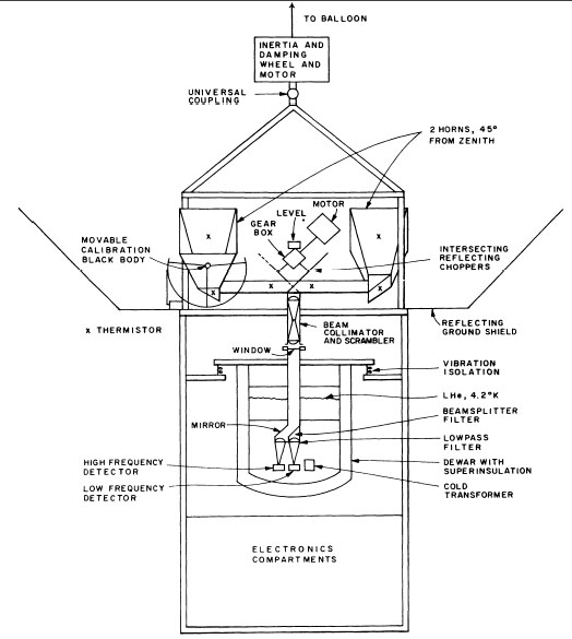Figure 11. A typical balloon-borne large angular scale isotropy experiment. This one is the M.I.T. instrument. The more successful Princeton balloon-borne instrument is similar in concept.

The signal is the difference in intensity measured in the two beams as a function of azimuth. The analysis is made by averaging this signal over a set of rotations occurring in the time it tales the celestial sphere to move about 1/2 a beam width. These averages are then expanded in a harmonic series in multiples of the rotation frequency. The fundamental component includes information on all multipole moments of the intensity distribution; higher odd harmonics exclude the leer order anisotropy moments and are a diagnostic for discriminating discrete sources. With beams 180° apart in azimuth, the apparatus is insensitive to even harmonic components although signals at these frequencies are valuable in diagnosing internal difficulties such as radio frequency interference and microphonics.

A dipole anisotropy of amplitude T_d pointing along _d (RA) and _d (dec) would produce a fundamental component with polar and equatorial projections given by

(16)

where and are the right ascension and declination of the zenith and EA is the elevation angle of the beams (45°). The best fit of Equation (16) to the data of Cheng et al. (1979) is shown in Figure 12.

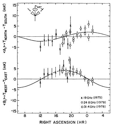Figure 12. The Princeton anisotropy measurements using a balloon platform. The best fit to a dipole anisotropy is shown as the solid line.

The balloon-borne observations were begun by Henry (1971) at 10 GHz. He measured the North-South component of the dipole anisotropy. The first definitive measurement (sufficient sky coverage and signal to noise) is that of Corey & Wilkinson (1976) at 19 GHz followed by the observation using the U2 airplane (Smoot et al. 1977) to be discussed below. Isotropy measurements in the spectral band embracing the blackbody peals, 3-10 cm^-1, were carried out from balloons by Muehlner and Weiss (Muehlner 1977). The data, perturbed by galactic dust emission, could only be used to set an upper limit on the dipole anisotropy. With unproved knowledge of the dust sources (Owens et al. 1979), the high frequency data has been reanalyzed, exhibiting a dipole anisotropy consistent with the lower frequency measurements (Muehlner & Weiss 1980). The spectrum of the dipole anisotropy appears to be close to Planckian.

The group at Berkeley (Smoot et al. 1977) has made good use of the U2 airplane as a platform to measure the large scale anisotropy. Although the airplane does not attain as high an altitude as the balloon, it offers some logistic advantages over the balloon, in particular in the relative ease of launching flights. The U2 instrument, Figure 13, is similar to the balloon-borne differential radiometers. It operates at 33 GHz and includes a 54 GHz radiometer to monitor the tilt of the airplane in the atmosphere. The radiometer beams are separated by 60° and are switched at 100 Hz. The entire apparatus is turned periodically within the airplane housing to measure intrinsic instrument anisotropies. Finally, the flights are arranged so as to observe the same regions of the shy with the airplane reversed in direction to account for anisotropies that might be fixed in the airplane coordinate system.

Figure 13. The U2 differential radiometer.

The observing and data analysis strategy (Gorenstein 1978, Gorenstein & Smoot 1980) is different than in the balloon experiments. Observation points in the sky are selected, Figure 14b and d, and the difference in intensity of the two beams is fit to a dipole distribution in a celestial coordinate system. The presentation of the data and the fit, Figure 14a and c, superposes all points that make the same polar angle with the dipole axis. Figure 14, as it stands, cannot be used to make a unique correspondence with a sky map.

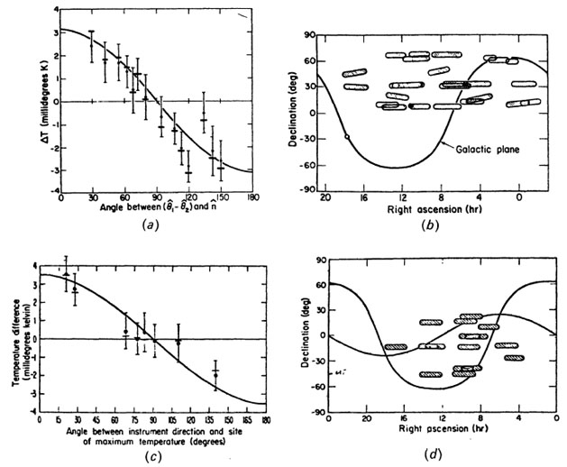Figure 14. The Berkeley anisotropy data using the U2 airplane. Panel a and c show the fit to the same dipole anisotropy using the data derived from sky coverage shown in b and d.

With the enhanced precision and more extended sky coverage of both the U2 (Smoot & Lubin 1979) and balloon experiments (Cheng et al. 1979), limits have been set on the five independent terms of a quadrupole moment of the CBR intensity distribution, Table 5. The balloon observations, all having been carried out at the same zenith declination, are not able to separate the polar dipole contribution, T_z, from the exclusively polar quadrupole term Q₁. Of the approximately 20 U2 flights that have been made, four were in the southern hemisphere specifically to break the correlation of these terms. The maximum magnitude of the quadrupole moment is less than 1 mK.

Table 5. Multipole fits of Berkeley and Princeton data (Lubin & Smoot 1979, Cheng et al. 1979)

Quadrupole and dipole fit
Princeton :
Berkeley :
	Berkeley	Princeton
Tx(mK)	-2.78±0.28	-3.27±0.57
Ty	+0.66±0.29	-0.17±0.73
Tz	-0.18±0.39	-0.10±0.72(Tz + 1.125Q1)
Q1	+0.38±0.26	-
Q2	+0.34±0.29	+0.22±0.50
Q3	+0.02±0.24	+0.26±0.67
Q4	-0.11±0.16	-0.05±0.36
Q5	+0.06±0.20	-0.22±0.38
Dipole fit only
Tx	-3.01±0.24	-2.98±0.30
Ty	+0.39±0.25	-0.24±0.30
Tz	+0.52±0.23	-0.06±0.31
T mK	3.1±0.4	2.99±0.34
°	9.6±6	-1±6
hr	11.4±0.4	12.3±0.4
v(2.7 K) km s-1	334±44	332±38
f(GHz)	33	19, 24.8, 31.4