G. Generalizations: III. Inhomogeneous density profiles

An interesting possibility that arose with the observation of the variable light curve of the afterglow of GRB 021004 is that the ejecta encounters surrounding matter with an irregular density profile [165, 209, 274]. To explore this situation one can resort to numerical simulation of the propagation of the blast wave into a selected density profile [209]. Instead one can attempt to model this analytically or almost analytically [271]. The key for this analytic model is the approximation of the light curve from an inhomogeneous density profile as a series of emission from instantaneous BM solutions, each with its own external density.

1. The light curve of a BM solution

The observed flux, at an observer time t, from an arbitrary spherically symmetric emitting region is given by [140]:

(98)

where n' is the emitters density and P' is the emitted spectral power per emitter, both are measured in the fluid frame; is the angle relative to the line of sight, and ^-1 = 1 / (1 - v cos / c) (v is the emitting matter bulk velocity) is the blue-shift factor.

Nakar and Piran [271] show ⁷ that using the self-similar nature of the BM profile (with an external density r^-k) one can reduce Eq. 98 to:

(99)

The integration over R is over the shock front of the BM solution. The upper limit R_max corresponds to the shock position from where photons leaving along the line of sight reach the observer at t. The factor D is the distance to the source (neglecting cosmological factors). is the local spectral index.

The factor g is a dimensionless factor that describes the observed pulse shape of an instantaneous emission from a BM profile. The instantaneous emission from a thin shell produces a finite pulse (see Section IVB and Fig. 14). This is generalized now to a pulse from an instantaneous emission from a BM profile. Note that even though the BM profile extends from 0 to R most of the emission arise from a narrow regions of width ~ R / ² behind the shock front. g is obtained by integration Eq. 98 over cos and r, i.e. over the volume of the BM profile. It depends only on the radial and angular structure of the shell. The self-similar profile of the shell enables us to express g as a general function that depends only on the dimensionless parameter (t - t_los(R)) / t_ang(R), with t_los(R) is the time in which a photon emitted at R along the line of sight to the center reaches the observer and t_ang R / 2c ². The second function, A, depends only on the conditions of the shock front along the line-of-sight. It includes only numerical parameters that remain after the integration over the volume of the shell.

When all the significant emission from the shell at radius R is within the same power-law segment, , (i.e is far from the break frequencies) then A and g are given by:

(100)

where R is the radius of the shock front, n_ext(R) is the external density, E is the energy in the blast-wave, M(R) the total collected mass up to radius R and H is a numerical factor which depends on the observed power law segment (see [271] for the numerical values.

(101)

where

(102)

This set of equations is completed with the relevant relations between the different variables of the blast wave, the observer time and the break frequencies.

These equations describe the light curve within one power law segment of the light curve. Matching between different power laws can be easily done [271]. The overall formalism can be used to calculate the complete light curve of a BM blast wave.

2. The light curve with a variable density or energy

The results of the previous section can be applied to study the effect of variations in the external density or in the energy of the blast-wave by approximating the solution as a series of instantaneous BM solutions whose parameters are determined by the instantaneous external density and the energy. Both can vary with time. This would be valid, of course, if the variations are not too rapid. The light curve can be expressed as an integral over the emission from a series of instantaneous BM solutions.

When a blast wave at radius R propagates into the circumburst medium, the emitting matter behind the shock is replenished within R R(2^{1 / (4 - k)} - 1). This is the length scale over which an external density variation relaxes to the BM solution. This approximation is valid as long as the density variations are on a larger length scales than R. It fails when there is a sharp density increase over a range of R. However, the contribution to the integral from the region on which the solution breaks is small (R / R << 1) and the overall light curve approximation is acceptable. Additionally the density variation must be mild enough so that it does not give rise to a strong reverse shock that destroys the BM profile.

A sharp density decrease is more complicated. Here the length scale in which the emitting matter behind the shock is replenished could be of the order of R. As an example we consider a sharp drop at some radius R_d and a constant density for R > R_d. In this case the external density is negligible at first, and the hot shell cools by adiabatic expansion. Later the forward shock becomes dominant again. Kumar and Panaitescu [204] show that immediately after the drop the light curve is dominated by the emission during the adiabatic cooling. Later the the observed flux is dominated by emission from R R_d, and at the end the new forward shock becomes dominant. Our approximation includes the emission before the density drop and the new forward shock after the drop, but it ignores the emission during the adiabatic cooling phase.

As an example for this method Fig 24 depicts the _m < < _c light curve for a Gaussian (R / R = 0.1) over-dense region in the ISM. Such a density profile may occur in a clumpy environment. The emission from a clump is similar to the emission from a spherically over-dense region as long as the clump's angular size is much larger than 1 / . Even a mild short length-scale, over-dense region (with a maximal over-density of 2) influences the light curve for a long duration (mainly due to the angular spreading). This duration depends strongly on the magnitude of the over-density.

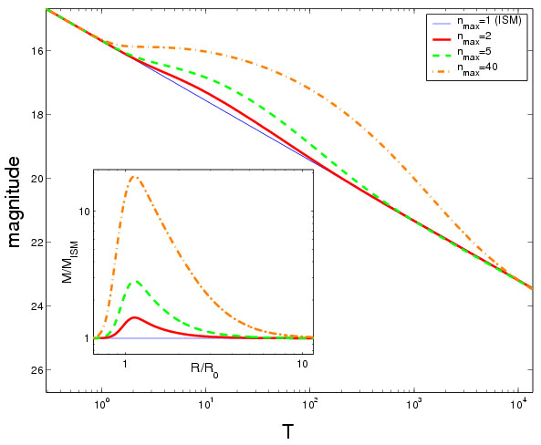Figure 24. The light curves results from a Gaussian (R / R = 0.1) over-dense region in the ISM. The different thick lines are for a maximal over-densities of 40 (dashed-dot), 5 (dashed) and 2 (solid). The thin line is the light curve for a constant ISM density. The inset depicts the ratio of the mass, M(R) over the mass of an ISM (without the over-dense region), MISM(R) (from Nakar and Piran [271])

The method can be applied also to variations in the blast wave's energy. Spherically symmetric energy variations are most likely to occur due to refreshed shocks, when new inner shells arrive from the source and refresh the blast wave [207, 335, 366]. Once more, this approximation misses the effect of the reverse shock that arise in this case [207]. However it enables a simple calculation of the observed light curve for a given energy profile.

⁷ See [140] for an alternative method for integrating Eq. 98. Back.