I. Generalizations: V. Angular Dependent Jets and the Structured Jet Model

In a realistic jet one can expect either a random or regular angular dependent structure. Here there are two dominant effects. As the ejecta slows down its Lorentz factor decreases and an observer will detect radiation from an angular region of size ^-1 (see Section IVC). At the same time the mixing within the ejecta will lead to an intrinsic averaging of the angular structure. Thus, both effects lead to an averaging over the angular structure at later times.

Several authors [219, 347, 446] suggested independently a different interpretation to the observed achromatic breaks in the afterglow light curves. This interpretation is based on a jet with a regular angular structure. According to this model all GRBs are produced by a jet with a fixed angular structure and the break corresponds to the viewing angle. Lipunov et al. [219] considered a "universal" jet with a 3-step profile: a spherical one, a 20° one and a 3° one. Rossi et al. [347] and Zhang and Mészáros [446] considered a special profile where the energy per solid angle, (), and the Lorentz factor (t = 0, ) are:

(106)

and

(107)

where _j is a maximal angle and core angle, _c, is introduced to avoid a divergence at = 0 and the parameters a and b here define the energy and Lorentz factor angular dependence. This core angle can be taken to be smaller than any other angle of interest. The power law index of , b, is not important for the dynamics of the fireball and the computation of the light curve as long as (t = 0, ) ₀() > ^-1 and ₀() >> 1.

To fit the constant energy result [105, 291, 310] Rossi et al. [347] consider a specific angular structure with a = 2. Rossi et al. [347] approximate the evolution assuming that at every angle the matter behaves as if it is a part of a regular BM profile (with the local and (t, )) until (t, ) = ^-1. Then the matter begins to expand sideways. The resulting light curve is calculated by averaging the detected light resulting from the different angles. They find that an observer at an angle _o will detect a break in the light curve that appears around the time that (t, _o) = _o^-1 (see Fig. 28). A simple explanation of break is the following: As the evolution proceeds and the Lorentz factor decreases an observer will detect emission from a larger and larger angular regions. Initially the additional higher energy at small angles, < _o compensates over the lower energies at larger angles > _o. Hence the observer detects a roughly constant energy per solid angle and the resulting light curve is comparable to the regular pre-jet break light curve. This goes on until ^-1(0) = _o. After this stage an further increase in the viewing angle ^-1 will result in a decrease of the energy per unit solid angle within the viewing cone and will lead to a break in the light curve.

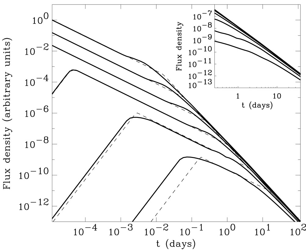Figure 28. The light curves of an inhomogeneous jet observed from different angles (From Rossi et al. [347]). From the top o = 0.5, 1, 2, 4, 8, 16°. The break time is related only to the observer angle: tb o2. The dashed line is the on-axis light curve of an homogeneous jet with an opening angle 2o and an energy per unit solid angle (o). The blow up is the time range between 4 hours and 1 month, where most of the optical observations are performed. Comparing the solid and the dashed lines for a fixed o, it is apparent that one can hardly distinguish the two models by fitting the afterglow data.

This interpretation of the breaks in the light curves in terms of the viewing angles of a standard structured jets implies a different understanding of total energy within GRB jets and of the rate of GRBs. The total energy in this model is also a constant but now it is larger as it is the integral of Eq. 106 over all viewing angles. The distribution of GRB luminosities, which is interpreted in the uniform jet interpretation as a distribution of jet opening angles is interpreted here as a distribution of viewing angles. As such this distribution is fixed by geometrical reasoning with P(_o) d_o sin_o d_o (up to the maximal observing angle _j). This leads to an implied isotropic energy distribution of

(108)

Guetta et al. [153] and Nakar et al. [266] find that these two distributions are somewhat inconsistent with current observations. However the present data that suffers from numerous observational biases is insufficient to reach a definite conclusions.

In order to estimate better the role of the hydrodynamics on the light curves of a structured jet Granot and Kumar [135], Granot et al. [136] considered two simple models for the hydrodynamics. In the first (model 1) there is no mixing among matter moving at different angles i.e. (, t) = (, t₀). In the second (model 2) is a function of time and it is averaged over the region to which a sound wave can propagate (this simulates the maximal lateral energy transfer that is consistent with causality). They consider various energy and Lorentz factors profiles and calculate the resulting light curves (see Fig. 29).

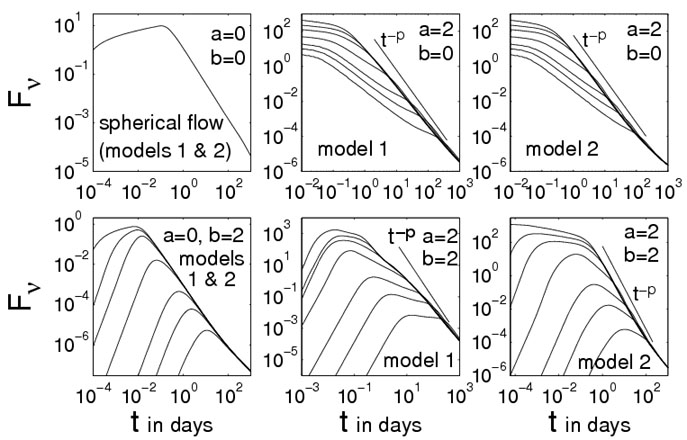Figure 29. Light curves for structured jets (initially -a and -b), for models 1 and 2, in the optical ( = 5 × 1014 Hz), for a jet core angle c = 0.02, viewing angles obs = 0.01, 0.03, 0.05, 0.1, 0.2, 0.3, 0.5, p = 2.5, e = B = 0.1, n = 1 cm-3, 0 = 103, and 0 was chosen so that the total energy of the jet would be 1052 erg (GK). A power law of t-p is added in some of the panels, for comparison. From Granot et al. [136]

Granot and Kumar [135] find that the light curves of models 1 and 2 are rather similar in spite of the different physical assumptions. This suggests that the widening of the viewing angle has a more dominant effect than the physical averaging. For models with a constant energy and a variable Lorentz factor ((a, b) = (0, 2)) the light curve initially rises and there is no jet break, which is quite different from observations for most afterglows. For (a, b) = (2, 2), (2, 0) they find a jet break at t_j when (_o) ~ _o^-1. For (a, b) = (2, 2) the value, ₁, of the temporal decay slope at t < t_j increases with _o, while ₂ = (t > t_j) decreases with _o. This effect is more prominent in model 1, and appears to a lesser extent in model 2. This suggests that = ₁ - ₂ should increase with t_j, which is not supported by observations. For (a, b) = (2, 0), there is a flattening of the light curve just before the jet break (also noticed by Rossi et al. [347]), for _o > 3_c. Again, this effect is larger in model 1, compared to model 2 and again this flattening is not seen in the observed data.

Clearly a full solution of an angular dependent jet requires full numerical simulations. Kumar and Granot [202] present a simple 1-D model for the hydrodynamics that is obtained by assuming axial symmetry and integrating over the radial profile of the flow, thus considerably reducing the computation time. The light curves that they find resemble those of models 1 and 2 above indicating that these crude approximations are useful. Furthermore they find relatively little change in () within the first few days, suggesting that model 1 is an especially useful approximation for the jet dynamics at early times, while model 2 provides a better approximation at late times.