J. Afterglow Polarization - a tool that distinguished between the different jet models

Synchrotron emission from a jet (in which the spherical symmetry is broken) would naturally produce polarized emission [126, 147, 365]. Moreover, the level and the direction of the polarization are expected to vary with time and to give observational clues on the geometrical structure of the emitting jet and our observing angle with respect to it.

The key feature in the determination of the polarization during the afterglow is the varying Lorentz factor and (after jet break) varying jet width. This changes changes the overall geometry (see Fig. 16) and hence the observer sees different geometries [177, 365]. Initially, the relativistic beaming angle 1 / is narrower than the physical size of the jet ₀, and the observer see a full ring and therefore the radial polarization averages out (the first frame, with ₀ = 4 of the left plot in Fig. 30). As the flow decelerates, the relativistic beaming angle 1 / becomes comparable to ₀ and only a fraction of the ring is visible; net polarization is then observed. Assuming, for simplicity, that the magnetic field is along the shock then the synchrotron polarization will be radially outwards. Due to the radial direction of the polarization from each fluid element, the total polarization is maximal when a quarter ( ₀ = 2 in Figure 30) or when three quarters ( ₀ = 1 in Figure 30) of the ring are missing (or radiate less efficiently) and vanishes for a full and a half ring. The polarization, when more than half of the ring is missing, is perpendicular to the polarization direction when less than half of it is missing.

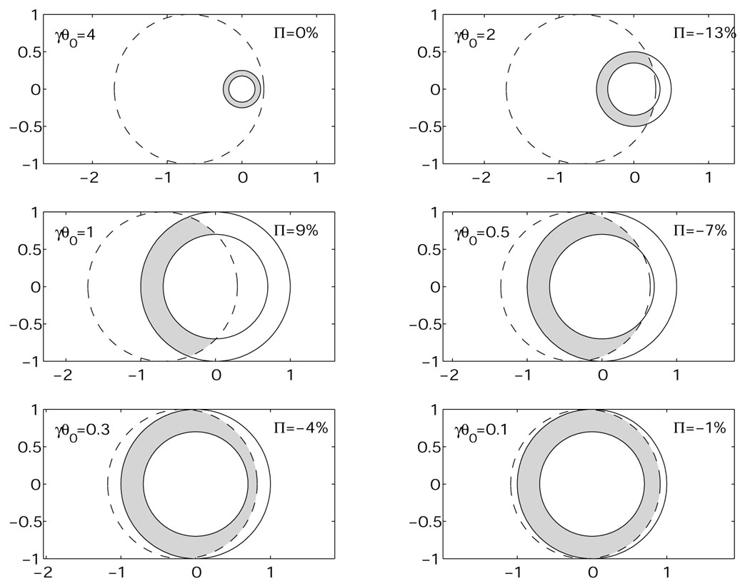
Figure 30. Top: Shape of the emitting region. The dashed line marks the physical extent of the jet, and solid lines give the viewable region 1 / . The observed radiation arises from the gray shaded region. In each frame, the percentage of polarization is given at the top right and the initial size of the jet relative to 1 / is given on the left. The frames are scaled so that the size of the jet is unity. Bottom: Observed and theoretical polarization light curves for three possible offsets of the observer relative to the jet axis Observational data for GRB 990510 is marked by crosses (x), assuming tjet = 1.2 days. The upper limit for GRB 990123 is given by a triangle, assuming tjet = 2.1 days (from [365]).

At late stages the jet expands sideways and since the offset of the observer from the physical center of the jet is constant, spherical symmetry is regained. The vanishing and re-occurrence of significant parts of the ring results in a unique prediction: there should be three peaks of polarization, with the polarization position angle during the central peak rotated by 90° with respect to the other two peaks. In case the observer is very close to the center, more than half of the ring is always observed, and therefore only a single direction of polarization is expected. A few possible polarization light curves are presented in Fig. 30.

The predicted polarization from a structured jet is drastically different from the one from a uniform jet, providing an excellent test between the two models [348]. Within the structured jet model the polarization arises due to the gradient in the emissivity. This gradient has a clear orientation. The emissivity is maximal at the center of center of the jet and is decreases monotonously outwards. The polarization will be maximal when the variation in the emissivity within the emitting beam are maximal. This happens around the jet break when _obs ~ ^-1 and the observed beam just reaches the center. The polarization expected in this case is around 20% [348] and it is slightly larger than the maximal polarization from a uniform jet. As the direction of the gradient is always the same (relative to a given observer) there should be no jumps in the direction of the polarization.

According to the patchy shell model [206] the jet can includes variable emitting hot spots. This could lead to a fluctuation in the light curve (as hot spots enter the observed beam) and also to corresponding fluctuations in the polarization [133, 267]. There is a clear prediction [267, 274] that if the fluctuations are angular fluctuations have a typical angular scale _f then the first bump in the light curve should take place on the time when ^-1 ~ _f (the whole hot spot will be within the observed beam). The following bumps in the light curve should decrease in amplitude (due to statistical fluctuations). Nakar and Oren [267] show analytically and numerically that the jumps in the polarization direction should be random, sharp and accompanied by jumps in the amount of polarization.