Annu. Rev. Astron. Astrophys. 2002. 40: 539-577 Copyright © 2002 by Annual Reviews. All rights reserved

4. THE SPACE DENSITY OF X-RAY CLUSTERS

4.1. Local Cluster Number Density

The determination of the local (z 0.3) cluster abundance plays a crucial role in assessing the evolution of the cluster abundance at higher redshifts. The cluster XLF is commonly modeled with a Schechter function:

(7)

where is the faint-end slope, L^*_X is the characteristic luminosity, and ^* is directly related to the space-density of clusters brighter than L_min: n₀ = _Lmin (L) dL. The cluster XLF in the literature is often written as: (L₄₄) = K exp(- L_X / L^*_X) L₄₄^-, with L₄₄ = L_X / 10⁴⁴ erg s^-1. The normalization K, expressed in units of 10^-7 Mpc^-3(10⁴⁴ erg s^-1)^-1, is related to ^* by ^* = K (L^*_X / 10⁴⁴)^1-.

Using a flux-limited cluster sample with measured redshifts and luminosities, a binned representation of the XLF can be obtained by adding the contribution to the space density of each cluster in a given luminosity bin L_X:

(8)

where V_max is the total search volume defined as

(9)

Here S(f) is the survey sky coverage, which depends on the flux f = L / (4 d_L²), d_L(z) is the luminosity distance, and H(z) is the Hubble constant at z (e.g. Peebles 1993, pag. 312). We define z_max as the maximum redshift out to which the object is included in the survey. Equations 8 and 9 can be easily generalized to compute the XLF in different redshift bins.

In Figure 6 we summarize the recent progress made in computing (L_X) using primarily low-redshift ROSAT based surveys. This work improved the first determination of the cluster XLF (Piccinotti et al. 1982, see Section 3.2). The BCS and REFLEX cover a large L_X range and have good statistics at the bright end, L_X L^*_X and near the knee of the XLF. Poor clusters and groups (L_X 10⁴³ erg s^-1) are better studied using deeper surveys, such as the RDCS. The very faint end of the XLF has been investigated using an optically selected, volume-complete sample of galaxy groups detected a posteriori in the RASS (Burns et al. 1996).

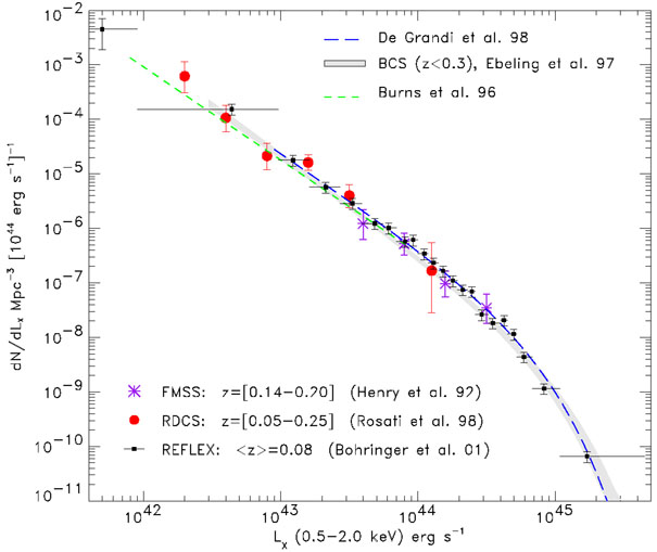Figure 6. Determinations of the local X-ray Luminosity Function of clusters from different samples (an Einstein-de-Sitter universe with H0 = 50 km s-1 Mpc-1 is adopted). For some of these surveys only best fit curves to XLFs are shown.

From Figure 6, we note the very good agreement among all these independent determinations. Best-fit parameters are consistent with each other with typical values: 1.8 (with 15% variation), ^* 1 × 10^-7 h₅₀³ Mpc^-3 (with 50% variation), and L^*_X 4 × 10⁴⁴ erg s^-1 [0.5-2 keV]. Residual differences at the faint end are probably the result of cosmic variance effects, because the lowest luminosity systems are detected at very low redshifts where the search volume becomes small (see Böhringer et al. 2002b). Such an overall agreement is quite remarkable considering that all these surveys used completely different selection techniques and independent datasets. Evidently, systematic effects associated with different selection functions are relatively small in current large cluster surveys. This situation is in contrast with that for the galaxy luminosity function in the nearby Universe, which is far from well established (Blanton et al. 2001). The observational study of cluster evolution has indeed several advantages respect to galaxy evolution, despite its smaller number statistics. First, a robust determination of the local XLF eases the task of measuring cluster evolution. Second, X-ray spectra constitute a single parameter family based on temperature and K-corrections are much easier to compute than in the case of different galaxy types in the optical bands.