7. LYMAN ALPHA EMITTERS AND GRAVITATIONAL LENSING

7.1. Strong Gravitational Lensing - A Primer

Slowly during the twentieth century, gravitational lensing moved from a curiosity associated with the verification of General Relativity (Eddington 1919) to a practical tool of cosmologists and those studying distant galaxies. There are many excellent reviews of both the pedagogical aspects of lensing (Blandford & Narayan 1998, Mellier 2000, Refregier 2003) and a previous Saas-Fee contributor (Schneider 2006).

To explore the distant Universe, we are primarily concerned with strong lensing - where the lens has a projected mass density, above a critical value, _crit, so that multiple images and high source magnifications are possible. For a simple thin lens

where D represents the angular diameter distance and the subscripts O,L,S refer to the observer, source and lens, respectively. Rather conveniently, for a lens at z 0.5 and a source at z > 2, the critical projected density is about 1 g cm^-2 - a value readily exceeded by most massive clusters. The merits of exploring the distant Universe by imaging through clusters was sketched in a remarkably prophetic article by Zwicky (1937).

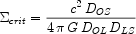
In lensing theory it is convenient to introduce a source plane, the true sky, and an image plane, the detector at our telescope, where the multiple images are seen. The relationship between the two is then a mapping transformation which depends on the relative distances (above). Crucially, what the observer sees depends on the degree of alignment between the source and lens as illustrated in Figure 46.

Figure 46. Configurations in the image plane for an elliptical lens as a function of the degree of alignment between the source and lens (second panel). Lines in the source plane refer to `caustics' which map to `critical lines' in the image plane (see text for details). (Courtesy of Jean-Paul Kneib)

An elliptical lens with > _crit for a given source and lens distance produces a pair of critical lines in the image plane where the multiple images lie. These lines map to caustics in the source plane. The outer critical line is equivalent to the Einstein radius _E

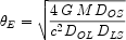and, for a given source and lens, is governed by the enclosed mass M. The location of the inner critical line depends on the gradient of the gravitational potential (Sand et al 2005).

The critical lines are important because they represent areas of sky where very high magnifications can be encountered - as high as ×30! For 20 well-studied clusters the location of these lines can be precisely determined for a given source redshift. Accordingly, it is practical to survey just those areas to secure a glimpse of otherwise inaccessibly faint sources boosted into view. The drawback is that, as in an optical lens, the sky area is similarly magnified, so the surface density of faint sources must be very large to yield any results. Regions where the magnification exceed ×10 are typically only 0.1-0.3 arcmin² per cluster in extent in the image plane and inconveniently shaped for most instruments (Figure 47). The sampled area in the source plane is then ten times smaller so to see even one magnified source/cluster requires a surface density of distant sources of ~ 50 arcmin^-2.

Figure 47. Hubble Space Telescope image of the rich cluster Abell 1689 with the critical lines for a source at z 5 overlaid in yellow. The narrow regions inbetween the pairs of yellow lines refer to regions where the magnification exceeds ×10.

Two other applications are particularly useful in faint galaxy studies. Firstly, strongly magnified systems at z 2-3 can provide remarkable insight into an already studied population by providing an apparently bright galaxy which is brought within reach of superior instrumentation. cB58, a Lyman break galaxy at z = 2.72 boosted by ×30 to V = 20.6 (Yee et al 1996, Seitz et al 1998) was the first distant galaxy to be studied with an echellette spectrograph (Pettini et al 2002), yielding chemical abundances and outflow dynamics of unprecedented precision.

More generally, a cluster can magnify a larger area of 2-4 arcmin² by a modest factor, say × 3-5. This has been effective in probing sub-mm source counts to the faintest possible limits (Smail et al 1997) and the method shows promise for similar extensions with the IRAC camera onboard Spitzer.

7.2. Creating a Cluster Mass Model

In the applications discussed above, in order to analyze the results, the inferred magnification clearly has to be determined. This will vary as a function of position in the cluster image and the relative distances of source and lens. The magnification follows from the construction of a mass model for the cluster.

The precepts for this method are discussed in the detailed analysis of the remarkable image of Abell 2218 taken with the WFPC-2 camera onboard HST in 1995 (Kneib et al 1996). An earlier image of AC 114 showed the important role HST would play in the recognition of multiple images (Smail et al 1995). Prior to HST, multiple images could only be located by searching for systems with similar colors, using the fact that lensing is an achromatic phenomenon. HST revealed that morphology is a valuable additional identifier; the improved resolution also reveals the local shear (see Figure 48).

Figure 48. Hubble Space Telescope study of the rich cluster AC114 (Smail et al 2005). (Top) Morphological recognition of a triply-imaged source. The lower inset panels zoom in on each of 3 images of the same source. (Bottom) Construction of mass contours (red lines) and associated shear (red vectors) from the geometrical arrangement of further multiple images labelled A1-3, B1-4, C1-3, Q1-3.

Today, various approaches are possible for constructing precise mass models for lensing clusters (Kneib et al 1996, Jullo et al 2006, Broadhurst et al 2005). These are generally based on utilizing the geometrical positions of sets of multiply-imaged systems whose redshift is known or assumed. This then maps the form and diameter of the critical line for a given z. Spectroscopic redshifts are particularly advantageous, as are pairs that straddle the critical line whose location can then be very precisely pinpointed. A particular mass model can be validated by `inverting' the technique and predicting the redshifts of other pairs prior to subsequent spectroscopy (Ebbels et al 1998).

The main debate among cognescenti in this area lies in the extent to which one should adopt a parametric approach to fitting the mass distribution, particularly in relation to the incorporation of mass clumps associated with individual cluster galaxy halos (Broadhurst et al 2005). Stark et al (2006b) discuss the likely uncertainties in the mass modeling process arising from the various techniques.

7.3. Lensing in Action: Some High z Examples

Before turning to Lyman emitters (lensed and unlensed), we will briefly discuss what has been learned from strongly-lensed dropouts.

Figure 49 shows a lensed pair in the cluster Abell 2218 (z = 0.18) as detected by NICMOS onboard HST and the two shortest wavelength channels of IRAC (Kneib et al 2004, Egami et al 2005). Although no spectroscopic redshift is yet available for this source, three images have been located by HST and their arrangement around the well-constrained z = 6 critical line suggests a source beyond z 6 (Kneib et al 2004).

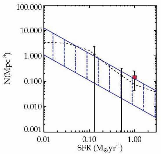Figure 49. (Top) Lensed pair of a z = 6.8 source as seen by NICMOS and IRAC in the rich cluster Abell 2218 (Egami et al 2005). The pair straddles the critical line at z 6 and a fainter third image at a location predicted by the lensing model has been successfully recovered in the HST data (Kneib et al 2004). (Bottom) Spectral energy distribution of the source revealing a significant Balmer break and improved estimates of the star formation rate, stellar mass and luminosity weighted age.

As with the unlensed i-band drop out studies by Eyles et al (2005) and Yan et al (2005), the prominent IRAC detections (Egami et al 2005) permit an improved photometric redshift and important constraints on the stellar mass and age. A redshift of z = 6.8 ± 0.1 is derived, independently of the geometric constraints used by Kneib et al. The stellar mass is 5-10 10⁸ M and the current star formation rate is 2.6 M yr^-1. The luminosity-weighted age corresponds to anything from 40-450 Myr for a normal IMF depending on the star formation history. Interestingly, the derived age for such a prominent Balmer break generally exceeds the e-folding timescale of the star formation history (Fig. 49) indicating the source would have been more luminous at redshifts 7 < z < 12 (unless obscured).

Given the small search area used to locate this object, such low mass sources may be very common. Accordingly, several groups are now surveying more lensing clusters for further examples of z band dropouts and even J-band dropouts (corresponding to z 8-10) . Richard et al are surveying 6 clusters with NICMOS and IRAC with deep ground-based K band imaging from Subaru and Keck. In these situations, one has to distinguish between magnifications of ×5 or so expected across the 2-3 arcmin fields of NICMOS and IRAC, and the much larger magnifications possible close to the critical lines. Contamination from foreground sources should be similar to what is seen in the GOODS surveys discussed in Lecture 6. The discovery of image pairs in the highly-magnified regions would be a significant step forward since spectroscopic confirmation of any sources at the limits being probed (H_AB 26.5-27.0) will be exceedingly difficult.

7.4. Lyman alpha Surveys

The origin and characteristic properties of the Lyman emission line has been discussed by my colleagues in their lectures (see also Miralda-Escude 1998, Haiman 2002, Barkana & Loeb 2004 and Santos 2004). The n = 2 to 1 transition corresponding to an energy difference of 10.2 eV and rest-wavelength of 1216 Å typically arises from ionizing photons absorbed by nearby hydrogen gas. The line has a number of interesting features which make it particularly well-suited for locating early star forming galaxies as well as for characterizing the nature of the IGM.

In searching for distant galaxies, emission lines offer far more contrast against the background sky than the faint stellar continuum of a drop-out. A line gives a convincing spectroscopic redshift (assuming it is correctly identified) and models suggest that as much as 7% of the bolometric output of young star-forming region might emerge in this line. For a normal IMF and no dust, a source with a star formation rate (SFR) of 1 M yr^-1 yields an emission line luminosity of 1.5 × 10⁴² ergs sec^-1.

Narrow band imaging techniques (see below) can reach fluxes of < 10^-17 cgs in comoving survey volumes of 10⁵ Mpc³, corresponding to a SFR 3 M yr^-1 at z 6. Spectroscopic techniques can probe fainter due to the improved contrast. This is particularly so along the critical lines where the additional boost of gravitational lensing enables fluxes as faint as 3 × 10^-19 cgs to be reached (corresponding to SFR 0.1 M yr^-1). However, in this case the survey volumes are much smaller ( 50 Mpc³). In this sense, the two techniques (discussed below) are usefully complementary.

Having a large dynamic range in surveys for Ly emission is important not just to probe the luminosity function of star-forming galaxies but also because it can be used to characterize the IGM. As a resonant transition, foreground hydrogen gas clouds can scatter away Ly photons in both direction and frequency. In a partially ionized IGM, scattering is maximum at 1216 Å in the rest-frame of the foreground cloud, thus affecting the blue wing of the observed line. However, in a fully neutral IGM, scattering far from resonance can occur leading to damping over the entire observed line. Figure 50 illustrates how, in a hypothetical situation where the IGM becomes substantially neutral during 6 < z < 7, surveys reaching the narrow-band flux limit would still find emitters at z = 7. Their intense emission would only be partially damped by even a neutral medium. However, lines with fluxes at the spectroscopic lensing limit would not survive. Accordingly, one possible signature of reionization would be a significant change in the shape of the Ly luminosity function at the faint end (Furlanetto et al 2005).

Figure 50. The Lyman damping wing is absorbed by neutral hydrogen and thus can act as a valuable tracer of the nature of the IGM. The simulation demonstrates the effect of HI damping on emission lines in high mass and low mass systems (characteristic of sources detected in typical narrow band and lensed spectroscopic surveys respectively) assuming reionization ends inbetween z = 6 and 7. The dramatic change in visibility of the weaker systems suggests their study with redshift may offer a sensitive probe of reionization. Courtesy: Mike Santos.

7.5. Results from Narrow Band Ly Surveys

The most impressive results to date have come from various narrow-band filters placed within the SuPrime camera at the prime focus of the Subaru 8m telescope (Kodaira et al 2003, Hu et al 2004, Ouchi et al 2005, Taniguchi et al 2005, Shimasaku et al 2005, Kashikawa et al 2006, Iye et al 2006). Important conclusions have also been deduced from an independent 4m campaign (Malhotra & Rhoads 2004).

Narrow band filters are typically manufactured at wavelengths where the night sky spectrum is quiescent, thus maximizing the contrast. These locations correspond to redshifts of z = 4.7, 5.7, 6.6 and 6.9 (Fig. 52). A recent triumph was the successful recovery of two candidates at z 6.96 by Iye et al (2006). Candidates are selected by comparing their narrow band fluxes with that in a broader band encompassing the narrow band wavelength range. The contrast can then be used as an indicator of line emission (Fig. 53). Spectroscopic follow-up is still desirable as the line could arise in a foregound galaxy with [O II] 3727 Å or [O III] 5007 Å emission. The former line is a doublet and the latter is part of a pair with a fixed line ratio, separated in the rest-frame by only 60 Å or so, so these contaminants are readily identified. Furthermore, Ly is often revealed by its asymmetric profile (c.f. Fig. 51).

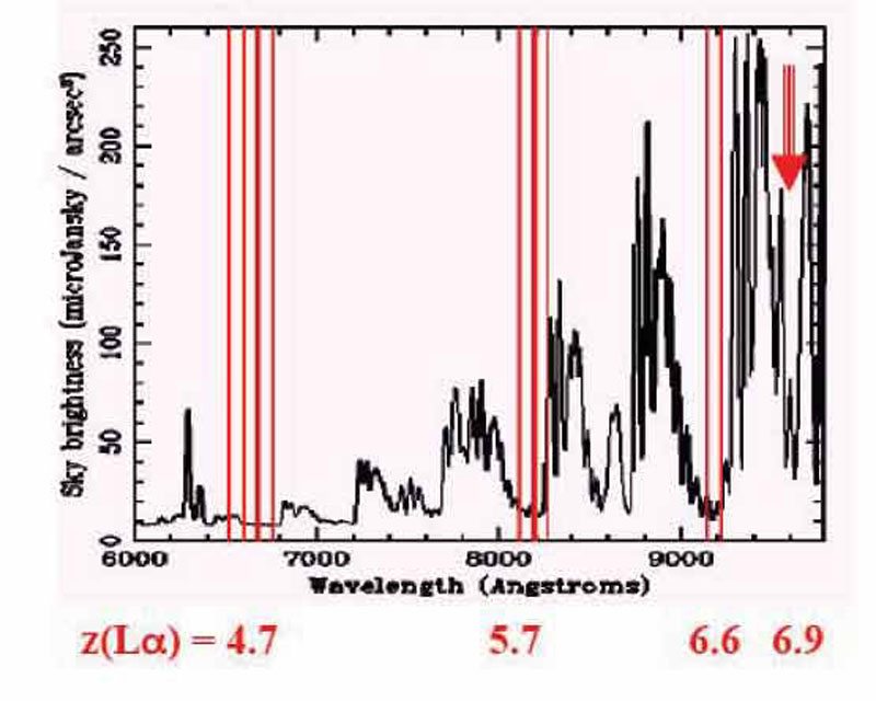Figure 51. Night sky spectrum and the deployment of narrow band filters in `quiet' regions corresponding to redshifted Lyman emission as indicated below. The final optical window, corresponding to z 6.9, was successfully exploited by Iye et al (2006) to find two sources close to z 7.

Figure 52. The two-step process for locating high redshift Lyman emitters (Hu et al 2004). (Left) Comparison of broad and narrow band magnitudes; sources with an unusual difference in the sense of being brighter in the narrow band filter represent promising candidates. (Right) Spectroscopic follow-up reveals typically three possibilities - [O III] or [O II] at lower redshift, or Ly often characterized by its asymmetric line profile.

Spectroscopic follow-up is obviously time-intensive for a large sample of candidates, hundreds of which can now be found with panoramic imagers such as SuPrimeCam. Therefore it is worth investigating additional ways of eliminating foreground sources. Tanuguchi et al (2005) combine the narrow band criteria adopted in Fig. 53 with a broad-band i - z drop-out signature. Spectroscopic follow-up of candidates located via this double color cut revealed a 50-70% success rate for locating high z emitters. The drawback is that the sources so found cannot easily be compared in number with other, more traditional, methods. Nagao et al (2005) used a narrow - broad band color criterion in the opposite sense, locating sources with a narrow band depression (rather than excess). Such rare sources are confirmed to be sources with extremely intense emission elsewhere in the broad-band filter. Such sources, with Lyman equivalent widths in excess of several hundred Å are interesting because they may challenge what can be produced from normal stellar populations.

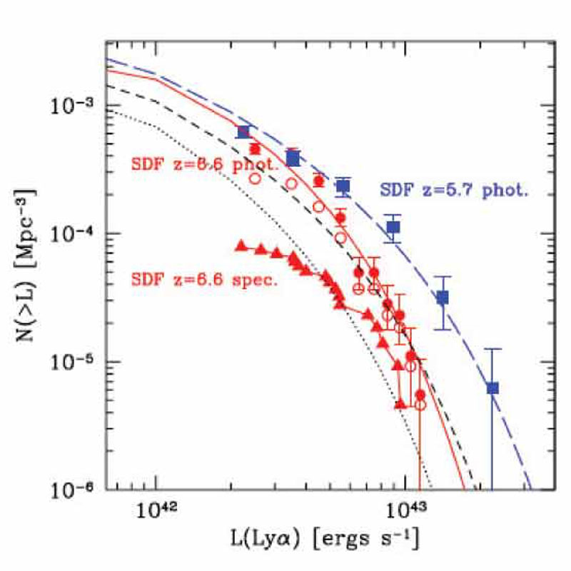Figure 53. Comparison of the Lyman luminosity functions at z = 5.7 and 6.5 from the surveys of Kashikawa et al (2006) and Shimasaku et al (2005); both spectroscopically-confirmed and photometric candidates are plotted. The decline in luminous emitters is qualitatively similar to trends seen over 3 < z < 6 in luminous continuum drop-outs.

Malhotra & Rhoads (2004) were the first to consider the absence of evolution in the Ly LF as a constraint on the neutral fraction. Although they found no convincing change in the LF between z = 5.7 and 6.5, the statistical uncertainties in both LFs were considerable. Specifically, below luminosities of L_Ly 10^42.5 ergs sec^-1 no detections were then available. Hu et al (2005) have also appealed to the absence of any significant change in the mean Ly profile. Malhotra & Rhoads deduced the neutral fraction must be x_HI < 0.3 at z 6 supporting early reionization. However, Furlanetto et al (2005) reanalyzed this constraint and indicated that strong emitters could persist even when x_HI 0.5 (c.f. Fig. 51).

Kashikawa et al (2006) and Shimasaku et al (2005) have determined statistically greatly improved Lyman luminosity functions and discuss both spectroscopic confirmed and photometrically-selected emitters (Fig. 53). No decline is apparent in the abundance of low luminosity emitters as expected in an IGM with high x_HI; indeed the most significant change is a decline with redshift in the abundance of the most luminous systems. Although the change seems surprisingly rapid given the time interval is only 150 Myr, this is consistent with growth in the halo mass function (Dijsktra et al 2006).

7.6. Results from Lensed Ly Surveys

The principal gain of narrow band imaging over other techniques in locating high redshift Lyman emitters lies in the ability to exploit panoramic cameras with fields of view as large as 30-60 arcmin. Since cosmic lenses only magnify fields of a few arcmin or less, lensing searches are only of practical utility when used in spectroscopic mode. As discussed above, the gain in sensitivity can be factors of ×30 or more, and given the small volumes explored, they are primarily useful in testing the faint end of the Ly luminosity function at various redshifts. A number of workers (e.g. Barkana & Loeb 2004) have emphasized the likelihood that the bulk of the reionizing photons arise from an abundant population of intrinsically-faint sources, and lensed searches provide the only practical route to observationally testing this hypothesis.

A practical demonstration of a blind search for lensed Ly emitters is summarized in Figure 54. A long slit is oriented along a straight portion of the critical line (whose location depends on the source redshift). The survey comprises several exposures taken in different positions offset perpendicular to the critical line. Candidate emission lines are astrometrically located on a deep HST image and, if a counter-image consistent with the mass model can be located, a separate exposure is undertaken to capture both (as was the case in the source located by Ellis et al 2001). Unfortunately, continuum emission is rarely seen from a faint emitter and the location of a corresponding second image is often too uncertain to warrant a separate search. In this case contamination from foreground sources has to be inferred from the absence of corresponding lines at other wavelengths (Santos et al 2004, Stark et al 2006b).

Figure 54. Critical line mapping in Abell 2218: how it works (Ellis et al 2001). The red curves show the location of the lines of very high magnification for a source at a redshift z=1 (dashed) and z = 6 (solid). Blue lines show the region scanned at low resolution with a long-slit spectrograph. The upper right panel shows the detection of an isolated line astrometrically associated with (a) in the HST image for which a counter image (b) is predicted and recovered (see also inset to main panel). A higher dispersion spectrum aligned between the pair (yellow lines) reveal strong emission with an asymmetric profile in both (lower right panel).

Using this technique with an optical spectrograph sensitive to Ly from 2.2 < z < 6.7, Santos et al (2004) conducted a survey of 9 lensing clusters and found 11 emitters probing luminosities as faint as L_Ly 10⁴⁰ cgs, significantly fainter than even the more recent Subaru narrow band imaging searches (Shimasaku et al 2006). The resulting luminosity function is flatter at the faint end than implied for the halo mass function and is consistent with suppression of star formation in the lowest mass halos.

Stark et al (2006b) have extended this technique to higher redshift using an infrared spectrograph operating in the J band, where lensed Ly emitters in the range 8.5 < z < 10.2 would be found. This is a much more demanding experiment than that conducted in the optical because of the brighter and more variable sky brightness, the smaller slit length necessitating very precise positioning to maximize the magnifications and, obviously, the fainter sources given the increased redshift. Nonetheless, a 5 sensitivity limit fainter than 10^-17 cgs corresponding to intrinsic (unlensed) star formation rates of 0.1 M yr^-1 is achieved with the 10m Keck II telescope in exposure times of 1.5 hours per slit position.

After surveying 10 clusters with several slit positions per cluster, 6 candidate emission lines have been found and, via additional spectroscopy, it seems most cannot be explained as foreground sources. Stark et al estimate the survey volume taking into account both the spatially-dependent magnification (from the cluster mass models) and the redshift-dependent survey sensitivity (governed by the night sky spectrum within the spectral band).

Madau et al (1999) and Stiavelli et al (2004) have introduced simple prescriptions for estimating the abundance of star forming sources necessary for cosmic reionizations. While these prescriptions are certainly simple-minded, given the coarse datasets at hand, they provide an illustration of the implications.

Generally, the abundance of sources of a given star formation rate SFR necessary for cosmic reionization over a time interval t is

where B is the number of ionizing photons required to keep a single hydrogen atom ionized, n_H is the comoving number density of hydrogen at the redshift of interest and f_c is the escape fraction of ionizing photons. Figure 55 shows the upshot of the Stark et al (2006b) survey for various assumptions. The detection of even a few convincing sources with SFR 0.1-1 M yr^-1 in such small cosmic volumes would imply a significant contribution from feeble emitters at z 10. Although speculative at this stage given both the uncertain nature of the lensed emitters and the calculation above, it nonetheless provides a strong incentive for continued searches.

Figure 55. The volume density of sources of various star formation rates at z 8-10 required for cosmic reionization for a range of assumed parameters (blue hatched region) compared to the inferred density of lensed emitters from the survey of Stark et al (2006b). The open red symbol corresponds to the case if all detected emitters are at z 10, the black symbols correspond to the situation if the two most promising candidates are at z 10, and the dashed line corresponds to the 5 upper limit if none of the candidates is at z 10.

7.7. Lecture Summary

In this lecture we have shown how Lyman emission offers more than simply a way to locate distant galaxies. The distribution of line profiles, equivalent widths and its luminosity function can act as a sensitive gauge of the neutral fraction because of the effects of scattering by hydrogen clouds. Surveys have been undertaken using optical cameras and narrow band filters to redshifts z 7.

However, despite great progress in the narrow-band surveys, as with the earlier i-band drop outs, there is some dispute as to the evolutionary trends being found. Surprisingly strong evolution is seen in luminous emitters over a very short period of cosmic time corresponding to 5.7 < z < 6.5. And, to date there is no convincing evidence that line profiles are evolving or that the equivalent width distribution of emitters is skewed beyond what can be accounted for by normal young stellar populations. One suspects we will have to push these techniques to higher redshift which will be hard given the Ly line moves into the infrared where no such panoramic instruments are yet available.

We have also given a brief tutorial on strong gravitational lensing. In about 20 or so clusters, spectroscopic redshifts for sets of multiple images has enabled quite precise mass models to be determined which, in turn, enable accurate magnification maps to be derived. Remarkably faint sources can be found by searching along the so-called critical lines where the magnification is high. The techniques has revealed a few intrinsically faint sources and, possibly, the first glimpse of a high abundance of faint star forming sources at z 10 has been secured.