6. INTO THE DARK AGES: LYMAN DROPOUTS

6.1. Motivation

Surveys of galaxies at and beyond a redshift z 6 represent the current observational frontier. We are motivated to search to conduct a census of the earliest galaxies seen 1 Gyr after the Big Bang as well as to evaluate the contribution of early star formation to cosmic reionization. Although impressive future facilities such as the next generation of extremely large telescope ⁶ and the James Webb Space Telescope (Gardner et al 2006) are destined to address these issues in considerable detail, any information we can glean on the abundance, luminosity and characteristics of distant sources will assist in planning their effective use.

In this lecture and the next, we will review the current optical and near-infrared techniques for surveying this largely uncharted region. They include

• Lyman dropouts: photometric searches based on locating the rest-frame ultraviolet continuum of star-forming sources introduced in Lecture 3. The key issue here is reducing contamination from foreground sources since most sources selected via this technique are too faint for confirmatory spectroscopy.

• Lyman alpha emitters: spectroscopic or narrow-band searches for sources with intense Ly emission. As the line is resonantly-scattered by neutral hydrogen its profile and strength gives additional information on the state of the high redshift intergalactic medium.

• Strong gravitational lensing: by coupling both above techniques with the magnification afforded by lensing clusters, it is possible to search for lower luminosity sources at high redshift. Since the magnified areas are small, the technique is only advantageous if the luminosity function has a steep faint end slope.

For the Lyman dropouts discussed here, as introduced in the last lecture, there is an increasingly important role played by the Spitzer Space Telescope in estimating stellar masses and earlier star formation histories.

The key questions we will address in this lecture focus on the (somewhat controversial) conclusions drawn from the analyses of Lyman dropouts thus far, namely:

1. How effective are the various high z selection methods? The characteristic luminosity L^* at z 6 corresponds to i_AB 26 where spectroscopic samples are inevitably biased to those with prominent Ly emission. Accordingly there is great reliance on photometric redshifts and a real danger of substantial contamination by foreground red galaxies and Galactic cool stars.

2. Is there a decline in the UV luminosity density, _UV, over the range 3 < z < 6? The early results were in some disagreement. Key issues relate to the degree of foreground contamination and cosmic variance in the very small deep fields being examined.

3. Is the observed UV density, _UV, at z 6 sufficient to account for reionization? The answer depends on the contribution from the faint end of the luminosity function and whether the UV continuum slope is steeper than predicted for a normal solar-metallicity population.

4. Significant stellar masses have been determined for several z 6 galaxies. Are these in conflict with hierarchical structure formation models?

6.2. Contamination in z 6 Dropout Samples

The traditional dropout technique exploited very effectively at z 3 (Lecture 3) is poorly suited for z 6 samples because the use of a simple i - z > 1.5 color cut still permits significant contamination by passive galaxies at z 2 and Galactic stars. The addition of an optical-infrared color allows some measure of discrimination (Stanway et al 2005) since a passive z 2 galaxy will be red over a wide range in wavelength, whereas a star-forming z 6 galaxy should be relatively blue in the optical-infrared color corresponding to its rest-frame ultraviolet (Figure 41). Application of this two color technique suggests contamination by foreground galaxies is 10% at the bright end (z_AB < 25.6) but negligible at the UDF limit (z_AB < 28.5)

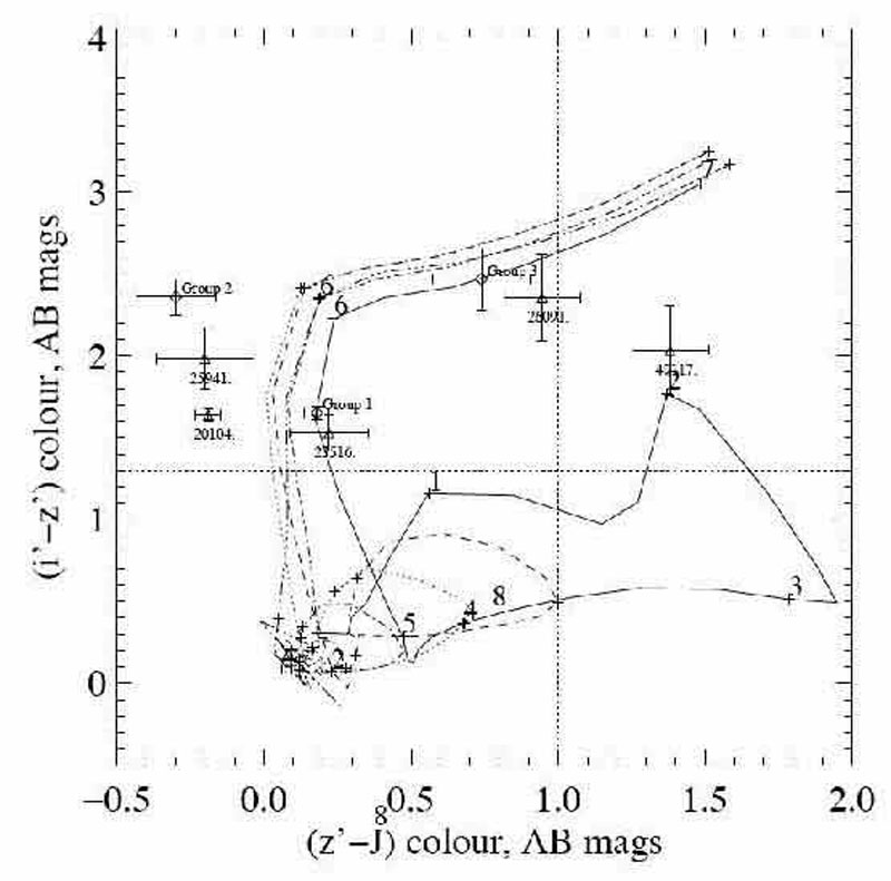Figure 41. The combination of a i - z and z - J color cut permits the distinction of z 5.7-6.5 star forming and z 2 passive galaxies. Both may satisfy the i - z > 1.5 dropout selector, but the former should lie blueward of the z - J = 1.0 divider, whereas z 2 are red in both colors. Crosses represent the location of candidates in the GOODS field and model tracks illlustrate the predicted colors for typical SEDs observed at the respective redshifts (Stanway et al 2005).

Unfortunately, the spectral properties of cool Galactic L dwarfs are dominated by prominent molecular bands rather than simply by their effective temperature. This means that they cannot be separated from z 6 galaxies in a similar color-color diagram. Indeed, annoyingly, these dwarfs occupy precisely the location of the wanted z 6 galaxies (Figure 42)! The only practical way to discriminate L dwarfs is either via spectroscopy or their unresolved nature in ACS images.

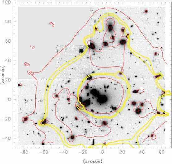Figure 42. (Left) Keck spectroscopic verification of two contaminating L dwarfs lying within the GOODS i - z dropout sample but pinpointed as likely to be stellar from ACS imaging data. The smoothed spectra represent high signal to noise brighter examples for comparison purposes. Strong molecular bands clearly mimic the Lyman dropout signature. (Right) Optical-infrared color diagram with the dropout color selector, iAB - zAB > 1.5, shown as the vertical dotted line. Bright L dwarfs (lozenges) frustratingly occupy a similar region of color space as the z 6 candidates (points with error bars) (Stanway et al 2004).

Stanway et al (2004) conducted the first comprehensive spectroscopic and ACS imaging survey of a GOODS i-drop sample limited at z_AB < 25.6, finding that stellar contamination at the bright end of the luminosity function of a traditional (i_AB - z_AB > 1.5) color cut could be as high as 30-40%. Unfortunately, even with substantial 6-8 hour integrations on the Keck telescope, redshift verification of the distant population was only possible in those dropout candidates with Ly emission. Stanway et al (2005) subsequently analyzed the ACS imaging properties of a fainter subset arguing that stellar contamination decreases with increasing apparent magnitude.

Further progress has been possible via the use of the ACS grism on board HST (Malhotra et al 2005). As the OH background is eliminated in space, despite its low resolution, it is possible even in the fairly low signal/noise data achievable with the modest 2.5m aperture of HST to separate a Lyman break from a stellar molecular band. It is claimed that of 29 z_AB < 27.5 candidates with (i - z) > 0.9, only 6 are likely to be low redshift interlopers.

Regrettably, as a result of these difficulties, it has become routine to rely entirely on photometric and angular size information without questioning further the degree of contamination. This is likely one reason why there remain significant discrepancies between independent assessments of the abundance of z 6 galaxies (Giavalisco et al 2004, Bouwens et al 2004, Bunker et al 2004). Although there are indications from the tests of Stanway et al (2004, 2005) and Malhotra et al (2005) that contamination is significant only at the bright end, the lack of a comprehensive understanding of stellar and foreground contamination remains a major uncertainty.

6.3. Cosmic Variance

The deepest data that has been searched for i-band dropouts includes the two GOODS fields (Dickinson et al 2004) and the Hubble Ultra Deep Field (UDF, Beckwith et al 2006). As these represent publicly-available fields they have been analyzed by many groups to various flux limits. The Bunker/Stanway team probed the GOODS fields to z_AB = 25.6 (spectroscopically) and 27.0 (photometrically, and the UDF to z_AB = 28.5. At these limits, it is instructive to consider the comoving cosmic volumes available in each field within the redshift range selected by the typical dropout criteria. For both GOODS-N/S fields, the total volume is 5 × 10⁵ Mpc³, whereas for the UDF it is only 2.6 × 10⁴ Mpc³. These contrast with 10⁶ Mpc³ for a single deep pointing taken with the SuPrime Camera on the Subaru 8m telescope.

Somerville et al (2004) present a formalism for estimating, for any population, the fractional uncertainty in the inferred number density from a survey of finite volume and angular extent. When the clustering signal is measurable, the cosmic variance can readily be calculated analytically. However, for frontier studies such as the i-dropouts, this is not the case. Here Somerville et al propose to estimate cosmic variance by appealing to the likely halo abundance for the given observed density using this to predict the clustering according to CDM models. In this way, the uncertainties in the inferred abundance of i-dropouts in the combined GOODS fields could be 20-25% whereas that in the UDF could be as high as 40-50%.

It seems these estimates of cosmic variance can only be strict lower limits to the actual fluctuations since Somerville et al make the assumption that halos containing star forming sources are visible at all times. If, for example, there is intermittent activity with some duty cycle whose "on/off" fraction is f, the cosmic variance will be underestimated by that factor f (Stark et al, in prep).

6.4. Evolution in the UV Luminosity Density 3 < z < 10?

The complementary survey depths means that combined studies of GOODS and UDF have been very effective in probing the shape of the UV luminosity function (LF) at z 6 ⁷. Even so, there has been a surprising variation in the derived faint end slope . Bunker et al (2004) claim their data (54 i-dropouts) is consistent with the modestly-steep = -1.6 found in the z 3 Lyman break samples (Steidel et 2003), whereas Yan & Windhorst (2004) extend the UDF counts to z_AB = 30.0 and, based on 108 candidates, find = -1.9, a value close to a divergent function! Issues of sample completeness are central to understanding whether the LF is this steep.

In a comprehensive analysis based on all the extant deep data, Bouwens et al (2006) have attempted to summarize the decline in rest-frame UV luminosity density over 3 < z < 10 as a function of luminosity (Figure 43). They attribute the earlier discrepancies noted between Giavalisco et al (2004), Bunker et al (2004) and Bouwens et al (2004) to a mixture of cosmic variance and differences in contamination and photometric selection. Interestingly, they claim a luminosity-dependent trend in the sense that the bulk of the decline occurs in the abundance of luminous dropouts, which they attribute to hierarchical growth.

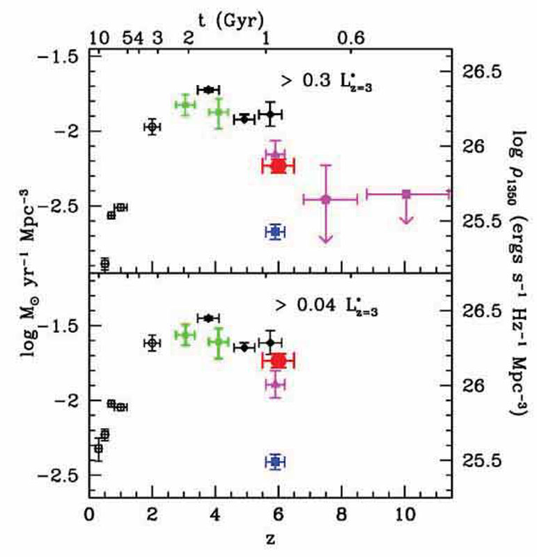Figure 43. Evolution in the rest-frame UV (1350 Å) luminosity density (right ordinate) and inferred star formation rate density ignoring extinction (left ordinate) for drop-out samples in two luminosity ranges from the compilation by Bouwens et al (2006). A marked decline is seen over 3 < z < 6 in the contribution of luminous sources.

A similar trend is seen in ground-based data obtained with Subaru. Although HST offers superior photometry and resolution which is effective in eliminating stellar contamination, the prime focus imager on Subaru has a much larger field of view so that each deep exposure covers a field twice as large as both GOODS N+S. As they do not have access to ACS data over such wide fields, the Japanese astronomers have approached the question of stellar contamination in an imaginative way. Shioya et al (2005) used two intermediate band filters at 709nm and 826nm to estimate stellar contamination in both z 5 and z 6 broad-band dropout samples. By considering the slope of the continuum inbetween these two intermediate bands, in addition to a standard i - z criterion, they claim an ability to separate L and T dwards. In a similar, but independent, study, Shimasaku et al (2005) split the z band into two intermediate filters thereby measuring the rest-frame UV slope just redward of the Lyman discontinuity. These studies confirm both the redshift decline and, to a lesser extent, the luminosity-dependent trends seen in the HST data.

Although it seems there is a 5× abundance decline in luminous UV emitting galaxies from z 3 to 6, it's worth noting again that the relevant counts refer to sources uncorrected for extinction. This is appropriate in evaluating the contribution of UV sources to the reionization process but not equivalent, necessarily, to a decline in the star formation rate density. Moreover, although the luminosity dependence seems similar in both ground and HST-based samples, it remains controversial (e.g. Beckwith et al 2006).

6.5. The Abundance of Star Forming Sources Necessary for Reionization

Have enough UV-emitting sources been found at z 6-10 to account for cosmic reionization? Notwithstanding the observational uncertainties evident in Figure 43, this has not prevented many teams from addressing this important question. The main difficulty lies in understanding the physical properties of the sources in question. The plain fact is that we cannot predict, sufficiently accurately, the UV luminosity density that is sufficient for reionization!

Some years ago, Madau, Haardt & Rees (1999) estimated the star formation rate density based on simple parameterized assumptions concerning the stellar IMF and/or metallicity Z essential for converting a 1350 Å luminosity into the integrated UV output, the fraction f_esc of escaping UV photons, the clumpiness of the surrounding intergalactic hydrogen, C = <_HI²> / <_HI>², and the temperature of the intergalactic medium T_IGM. In general terms, for reionization peaking at a redshift z_reion, the necessary density of sources goes as:

For likely ranges in each of these parameters, Stiavelli et al (2004) tabulate the required source surface density which, generally speaking, lie above those observed at z 6 (e.g. Bunker et al 2004).

It is certainly possible to reconcile the end of the reionization at z 6 with this low density of sources (Figure 43) by appealing to cosmic variance, a low metallicity and/or top-heavy IMF (Stiavelli et al 2005) or a steep faint end slope of the luminosity function (Yan & Windhorst 2004) but none of these arguments is convincing without further proof. As we will see, the most logical way to proceed is to explore both the extent of earlier star formation from the mass assembled at z 5-6 (Lecture 5) and to directly measure, if possible, the abundance of low luminosity sources at higher redshift.

6.6. The Spitzer Space Telescope Revolution: Stellar Masses at z 6

One of the most remarkable aspects of our search for the most distant and early landmarks in cosmic history is that a modest cooled 85cm telescope, the Spitzer Space Telescope, can not only assist but provide crucial diagnostic data! The key instrument is the InfraRed Array Camera (IRAC) which offers four channels at 3.6, 4.5, 5.8 and 8 µm corresponding to the rest-frame optical 0.5-1 µm at redshifts z 6-7. In the space of only a year, the subject has progressed from the determination of stellar masses for a few z 5-7 sources to mass densities and direct constraints on the amount of early activity, as discussed in Lecture 5.

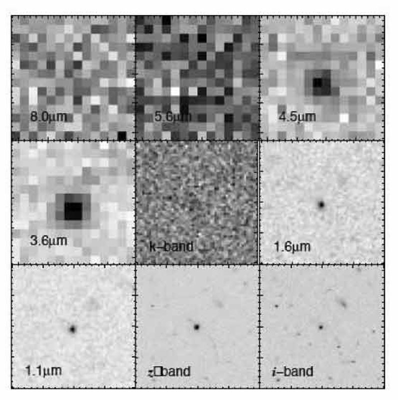
An early demonstration of the promise of IRAC in this area was provided by Eyles et al (2005) who detected two spectroscopically-confirmed z 5.8 i-band dropouts at 3.6 µm, demonstrating the presence of a strong Balmer break in their spectral energy distributions (Figure 44). In these sources, the optical detection of Ly emission provides an estimate of the current ongoing star formation rate, whereas the flux longward of the Balmer break provides a measure of the past averaged activity. The combination gives a measure of the luminosity weighted age of the stellar population. In general terms, a Balmer break appears in stars whose age cannot, even in short burst of activity, be younger than 100 Myr. Eyles et al showed such systems could well be much older (250-650 Myr) depending on the assumed form of the past activity. As the Universe is only 1 Gyr old at z 6, the IRAC detections gave the first indirect glimpse of significant earlier star formation - a glimpse that was elusive with direct searches at the time.

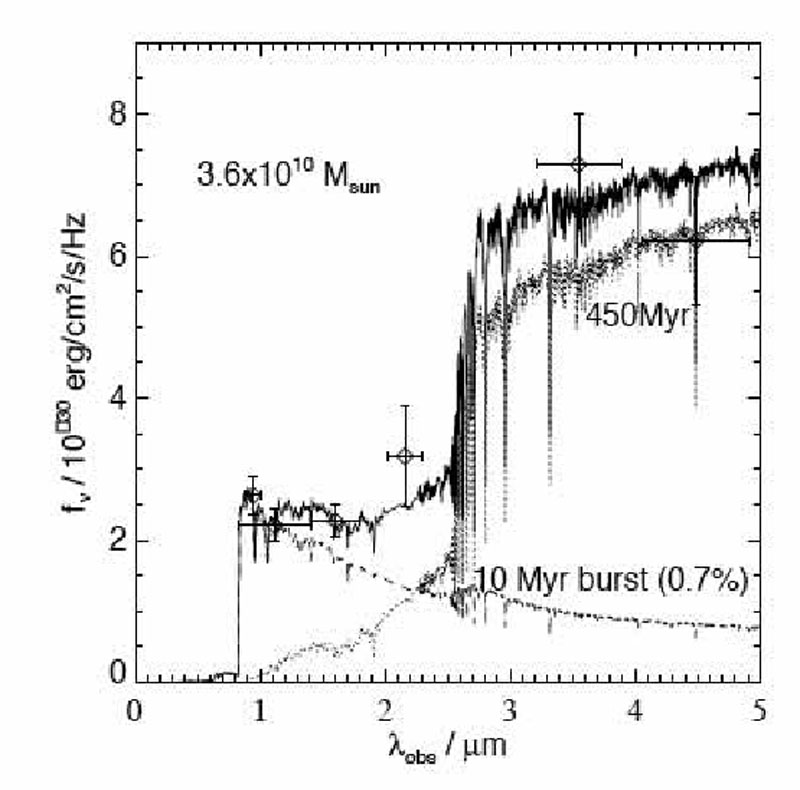Figure 44. (Left) Detection of a spectroscopically-confirmed i-drop at z = 5.83 from the analysis of Eyles et al (2005). (Right) Spectral energy distribution of the same source. Data points refer to IRAC at 3.6 and 4.5 µm, VLT (K) and HST NICMOS (J,H) overplotted on a synthesised spectrum; note the prominent Balmer break. Synthesis models indicate the Balmer break takes 100 Myr to establish. However, the luminosity-weighted age could be significantly older depending on the assumed past star formation rate. In the example shown, a dominant 450 Myr component (zF ~ 10) is rejuvenated with a more recent secondary burst whose ongoing star formation rate is consistent with the Ly flux observed in the source.

Independent confirmation of both the high stellar masses and prominent Balmer breaks was provided by the analysis of Yan et al (2005) who studied 3 z 5.9 sources. Moreover, Yan et al also showed several objects had (z - J) colors bluer than the predictions of the Bruzual-Charlot models for all reasonable model choices - a point first noted by Stanway et al (2004).

Eyles et al and Yan et al proposed the presence of established stellar populations in z 6 i-drops and also to highlight the high stellar masses (M 1 - 4 × 10¹⁰ M) they derived. At first sight, the presence of z 6 sources as massive as the Milky Way seems a surprising result. Yan et al discuss the question in some detail and conclude the abundance of such massive objects is not inconsistent with hierarchical theory. In actuality it is hard to be sure because cosmic variance permits a huge range in the derived volume density and theory predicts the halo abundance (e.g. Barkana & Loeb 2000) rather than the stellar mass density. To convert one into the other requires a knowledge of the star formation efficiency and its associated duty-cycle.

One early UDF source detected by IRAC has been a particular source of puzzlement. Mobasher et al (2005) found a J-dropout candidate with a prominent detection in all 4 IRAC bandpasses. Its photometric redshift was claimed to be z 6.5 on the basis of both a Balmer and a Lyman break. However, despite exhaustive efforts, its redshift has not been confirmed spectroscopically. The inferred stellar mass is 2-7 × 10¹¹ M, almost an order of magnitude larger than the spectroscopically-confirmed sources studied by Eyles et al and Yan et al. If this source is truly at z 6.5, finding such a massive galaxy whose star formation likely peaked before z 9 is very surprising in the context of contemporary hierarchical models. Such sources should be extremely rare so finding one in the tiny area of the UDF is all the more puzzling. Dunlop et al (2006) have proposed the source must be foreground both on account of an ambiguity in the photometric redshift determination and the absence of similarly massive sources in a panoramic survey being conducted at UKIRT (McClure et al 2006).

This year, the first estimates of the stellar mass density at z 5-6 have been derived (Yan et al 2006, Stark et al 2006a, Eyles et al 2006). Although the independenty-derived results are consistent, both with one another and with lower redshift estimates (Figure 45) the uncertainties are considerable as discussed briefly in the previous lecture. There are four major challenges to undertaking a census of the star formation at early times.

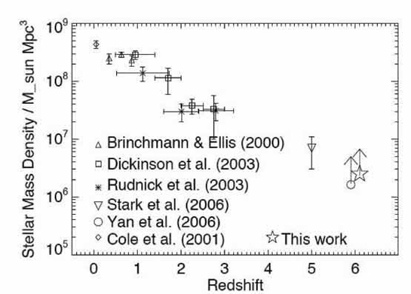Figure 45. Evolution in the comoving stellar mass density from the compilation derived by Eyles et al (2006). The recent z 5-6 estiimates constitute lower limits given the likelihood of quiescent sources missed by the drop-out selection technique. Results at z 6 are offset slightly in redshift for clarity.

Finally, as with all stellar mass determinations, many assumptions are made about the nature of the stellar populations involved and their star formation histories. Until individual z 5-6 sources can be studied in more detail, perhaps via the location of one or two strongly lensed examples, or via future more powerful facilities, this will regrettably remain the situation. At present, such density estimates are unlikely to be accurate to better than a factor of 2. Even so, they provide good evidence for significant earlier star formation (Stark et al 2006a, Lecture 5).

6.7. Lecture Summary

In this lecture we have discussed the great progress made in using v, i, z and J band Lyman dropouts to probe the abundance of star forming galaxies over 3 < z < 10. At redshifts z 6 alone, Bouwens et al (2006) discuss the properties of a catalog of 506 sources to z_AB = 29.5.

In practice, the good statistics are tempered by uncertain contamination from foreground cool stars and dusty or passively-evolving red z 2 galaxies and the vagaries of cosmic variance in the small fields studied. It may be that we will not overcome these difficulties until we have larger ground-based telescopes.

Nonetheless, from the evidence at hand, it seems that the comoving UV luminosity density declines from z 3 to 10, and that only by appealing to special circumstances can the low abundance of star forming galaxies at z > 6 be reconciled with that necessary to reionize the Universe.

One obvious caveat is our poor knowledge of the contribution from lower luminosity systems. Some authors (Yan & Windhorst 2004, Bouwens et al 2006) have suggested a steepening of the luminosity function at higher redshift. Testing this assumption with lensed searches is the subject of our next lecture.

Finally, we have seen the successful emergence of the Spitzer Space Telescope as an important tool in confirming the need for star formation at z > 6. Large numbers of z 5-6 galaxies have now been detected by IRAC. The prominent Balmer breaks and high stellar masses argue for much earlier activity. Reconciling the present of mature galaxies at z 6 with the absence of significant star formation beyond, is one of the most interesting challenges at the present time.

⁶ e.g. The US-Canadian Thirty Meter Telescope - http://www.tmt.org. Back.

⁷ In this section we will only refer to the observed (extincted) LFs and luminosity density. Back.