3. DISTANCE MEASURES

Distance measurements as a function of scale factor or redshift directly map the expansion history. Here we consider several approaches to these measurements, starting with the geometric or mostly geometric methods that give the cleanest probes of the expansion. Many other techniques involving distances exist, also containing noncosmological quantities. One can categorize probes into ones depending (almost) exclusively on geometry, ones requiring some knowledge of the mass of objects to separate out the distance dependence, and ones requiring not only knowledge of mass but the thermodynamic or hydrodynamical state of the material, i.e. mass+gas probes. The discussion here focuses on the geometric distance techniques actually implemented to date, though we do briefly mention some other approaches.

3.1. General cosmological distance properties

Because distances are integrals over the expansion history, which in turn involves an integral over the equation of state, degeneracies exist between cosmological parameters contributing to the distance. These are common to all distance measurements. Figures 7 - 8 illustrate the sensitivity and degeneracy of various expansion history measurements to the cosmological parameters. Here d is the luminosity or angular distance (we consider fractional precisions so the distinguishing factor of (1 + z)² cancels out), H is the Hubble parameter, or expansion rate, and the quantities = d(_m h²)^1/2, = H / (_m h²)^1/2, where h is the dimensionless Hubble constant, are relative to high redshift.

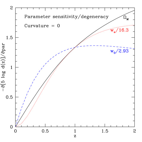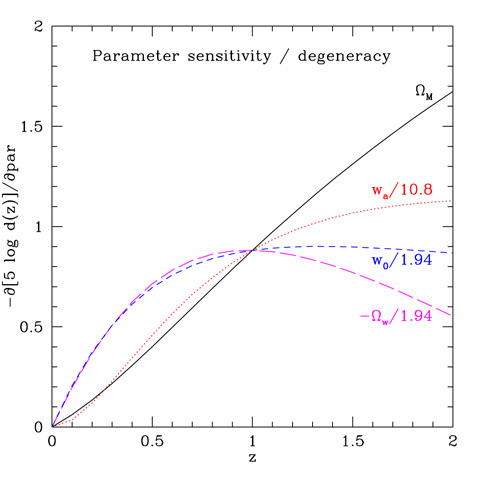
Figure 7. Fisher sensitivities for the magnitude (5 logd) are plotted vs. redshift for the case leaving spatial curvature free (left panel) and fixing it to zero, i.e. a flat universe (right panel). Since only the shapes of the curves matter for degeneracy, parameters are normalized to make this more evident. Observations out to z 1.5 are required to break the degeneracies.

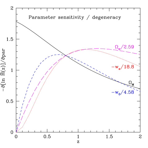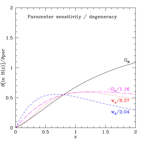
Figure 8. Fisher sensitivities for the Hubble parameter H (left panel) and reduced Hubble parameter = H / (m h2)1/2, i.e. Hubble parameter relative to high redshift (right panel), are plotted vs. redshift, leaving spatial curvature free. The behavior is similar to that in Figure 7 but the degeneracies are somewhat more severe.

First we note that for a given fractional measurement precision, distances contain about as much information as the Hubble parameter, despite the extra integral (the greater lever arm acts to compensate for the integral). That is (assuming flatness for simplicity),

(6) (7)

for a parameter , where angle brackets denote the weighted average. However, surveys to measure distances to a given precision can be much less time consuming than those to measure the Hubble parameter.

Concerning the physical interpretation of the partial derivatives, sometimes known as Fisher sensitivities since they also enter the Fisher information matrix [40], recall that

(8)

If for some parameter the Fisher partial derivative at some redshift is 0.88, say, then a 1% measurement gives an unmarginalized uncertainty on the parameter of 0.011. If the parameter is w_a / 10.8, say, this means the unmarginalized uncertainty on w_a is 0.12. The higher the denominator in the parameter label, the less sensitivity exists to that parameter.

The greatest sensitivity is to the energy densities in matter and dark energy; note that we do not here assume a flat universe. The nature of the dark energy is here described through the equation of state parametrization w(a) = w₀ + w_a(1 - a), where w₀ is the present value and w_a provides a measure of its time variation (also see Section 5.1). This has been shown to be an excellent approximation to a wide variety of origins for the acceleration [41]. Sensitivity to w_a is quite modest so highly accurate measurements are required to discover the physics behind acceleration.

Note that degeneracies between parameters, e.g. _m and w_a, and _w and w₀, are strong at redshifts z 1. Not until z > 1.5 do distance measurements make an appreciable distinction between these variables. This determines the need for mapping the expansion history over approximately the last e-fold of expansion, i.e. to a = 1 / e or z = 1.7. Since the flux of distant sources gets redshifted, this requires many observations to move into the near infrared, which can only be achieved to great accuracy from space.

From the right panel of Figure 7 we see that the degeneracy between the matter density _m and dark energy equation of state time variation w_a holds regardless of whether space is assumed flat or not. The dark energy density _w and the dark energy present equation of state w₀ stay highly degenerate in the curvature free case, whether considering d or (not shown in the figure).

From the relation between the derivatives of the distance with respect to cosmological parameters, as a function of redshift, one can intuit the orientation of confidence contours in various planes. For example, the sensitivity for the matter density and dark energy density enter with opposite signs, so increasing one can be compensated by increasing the other, explaining the low densities to high densities diagonal orientation in the _m - plane. Since the sensitivity to _m trends monotonically with redshift, while that of _w has a different shape, this implies that observations over a range of redshifts will rotate the confidence contours, breaking the degeneracies and tightening the constraints beyond the mere power of added statistics. Similarly one can see that contours in the _m - w₀ plane will have negative slope, as will those in the w₀ - w_a plane.

For the tilde variable , that is distances relative to high redshift rather than low redshift, there is relatively little degeneracy between the matter density and the other variables - but there is also much less sensitivity to the other variables. The equivalent normalized variables to those in the top left panel of Figure 7 are _w / 6.60, -w₀ / 6.59, and -w_a / 36.7. This insensitivity is why contours in the _m - _w or _m - w planes are rather vertical for distances tied to high redshift, like baryon acoustic oscillations. Of course since the degeneracy directions between distances tied to low redshift and those tied to high redshift are different, these measurements are complementary. (Although not as much in the w₀ - w_a plane, since high redshift is essentially blind to these parameters so tilde and regular distances have the same dependence.)

For the Hubble parameter, a nearly triple degeneracy exists between _m, _w and w_a out to z 1. Interestingly, for there is a strong degeneracy between _m and w₀ for z 1-2, while the _w - w_a degeneracy remains. It is quite difficult to observe H(z) directly, i.e. measured relative to low redshift; more common is measurement relative to high redshift as through baryon acoustic oscillation in the line of sight direction (see Section 3.4). Here, the sensitivity to the dark energy equation of state is reduced relative to the distance case, even apart from the degeneracies (since does not include the z 1 lever arm).

For either or the correlation between energy densities is reversed from the regular quantities, so the likelihood contour orientation in the _m - plane is reversed as well, close to that of the CMB, another measurement tied to the high redshift universe. The contour in _m - w₀ is similarly reversed but not in w₀ - w_a. Thus, all these varieties of distance measurements have similar equation of state dependencies and, unfortunately, no substantial orthogonality can be achieved in this plane.

To emphasize this last point, Figure 9 illustrates the degeneracy directions for contours of constant Hubble parameter and constant matter density at various redshifts. As we consider redshifts running from z = 0 to z >> 1, the isocontours only rotate moderately. Since they always remain oriented in the same quadrant, orthogonality is not possible.

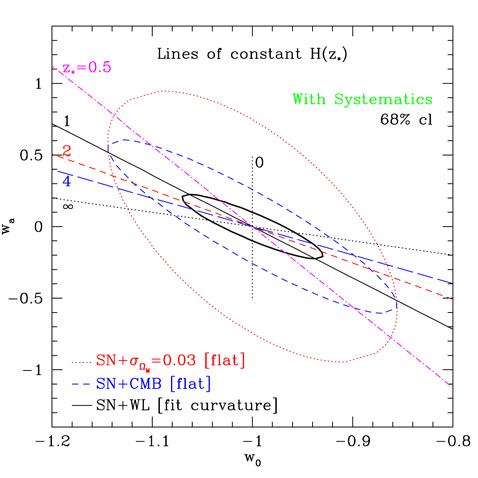Figure 9. Lines of constant expansion history, i.e. Hubble parameter, are plotted in the dark energy equation of state plane. Observations over a range of redshifts give complementarity, but never complete orthogonality. Contours show approximate examples of how certain combinations of distance probes effectively map different parts of the expansion history.

In this subsection we have seen that a considerable part of the optimal approach for mapping the expansion history is set purely by the innate cosmological dependence, and the survey design must follow these foundations as basic science requirements. The purpose of detailed design of successful surveys is rather to work within this framework to minimize systematic uncertainties in the measurements, discussed in more detail in Section 5. These two requirements give some of the main conclusions of this review.

3.2. Type Ia supernovae

The class of exploding stars called Type Ia supernovae (SN) become as bright as a galaxy and can be seen to great distances. Moreover, while having a modest intrinsic scatter in luminosity, they can be further calibrated to serve as standardized candles. Used in this way as distance measures, studies of SN led to the discovery of the acceleration of the universe [3, 4].

As of the beginning of 2008, over 300 SN with measurement quality suitable for cosmological constraints had been published, representing the efforts of several survey groups. Finding a SN is merely the first step: the time series of flux (the lightcurve), must be measured with high signal to noise from before peak flux (maximum light) to a month or more afterward. This must be done for multiple wavelength bands to permit dust and intrinsic color corrections. Additionally, spectroscopy to provide an accurate redshift and confirmation that it is a Type Ia supernova must be obtained. See [42] for further observational issues. (Also see [43] for the use of Type II-P supernovae.)

Once the multiwavelength fits and corrections are carried out, one derives the distance, often spoken of in terms of the equivalent magnitude or logarithmic flux known as the distance modulus. The distance-redshift or magnitude-redshift relation is referred to as the Hubble diagram. This, or any other derived distance relation, can then be compared to cosmological models.

Analysis of the world SN data sets published as of the start of 2008, comprising 307 SN, show the expansion history is consistent with a cosmological constant plus matter universe, CDM, but also with a great variety of other models [44]. Essentially no constraints on dark energy can be placed at z > 1 and the limits on time variation are no more stringent than the characteristic time scale being of the Hubble time or shorter. 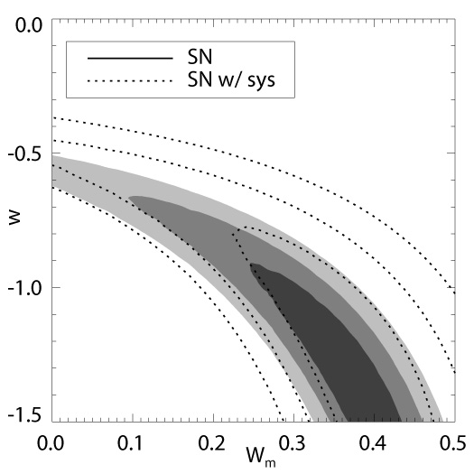Figure 10 shows that even for a flat universe and constant equation of state there is considerable latitude in dark energy characteristics and that systematic uncertainties need to be reduced for further numbers of SN to be useful.

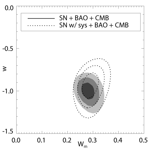Figure 10. 68.3%, 95.4%, and 99.7% confidence level contours on the matter density and constant equation of state from the Union 2007 set of supernova distances. The left panel shows SN only and the right panel includes current CMB and baryon acoustic oscillation constraints. From [44].

3.3. Cosmic microwave background

The geometric distance information within the cosmic microwave background radiation (CMB) arises from the angular scale of the acoustic peaks in the temperature power spectrum, reflecting the sound horizon of perturbations in the tightly coupled photon-baryon fluid at the time of recombination. If one can predict from atomic physics the sound horizon scale then it can be used as a standard ruler, with the angular scale then measuring the ratio of the sound horizon s to the distance to CMB last scattering at z_lss 1089. Related, but not identical to the inverse of this distance ratio, R = (_m h²)^1/2d_lss is often called the reduced distance or CMB shift parameter. This gives a good approximation to the full CMB leverage on the cosmic expansion for models near CDM [45]; for nonstandard models where the sound horizon is affected, this needs to be corrected [44] or supplemented [46].

Because the CMB essentially delivers a single distance, it cannot effectively break degeneracies between cosmological parameters on its own. While some leverage comes from other aspects than the geometric shift factor (such as the integrated Sachs-Wolfe effect), the dark energy constraints tend to be weak. However, as a high redshift distance indicator the CMB does provide a long lever arm useful for combination with other distance probes (effectively the z = line in Figure 9), and can strongly aid in breaking degeneracies [47].

The reduced distance to last scattering, being measured with excellent precision - 1.8% in the case of current data and the possibility of 0.4% precision with Planck data - defines a thin surface in cosmological parameter space (see, e.g., [48]). From Figure 11 we see that the acoustic peak structure contains substantial geometric information for mapping the cosmological expansion. This will provide most of the information on dark energy since cosmic variance prevents the low multipoles from providing substantial leverage (and almost none at all to the geometric quantities, as shown by the similarity of dashed and solid contours). Polarization information from E-modes and the cross spectrum improves the geometric knowledge. The distance ratio d_lss / s of the distance to last scattering relative to the sound horizon is determined much better (almost 20 times so) than the reduced distance to last scattering R = (_m h²)^1/2d_lss, but there is substantial covariance between these quantities (as evident in the right panel) for models near CDM (unless broken through external priors on, e.g., the Hubble constant).

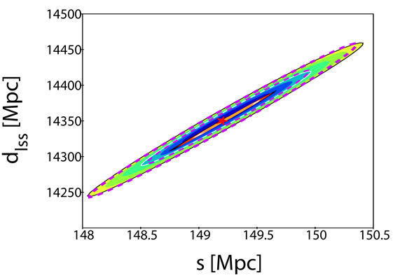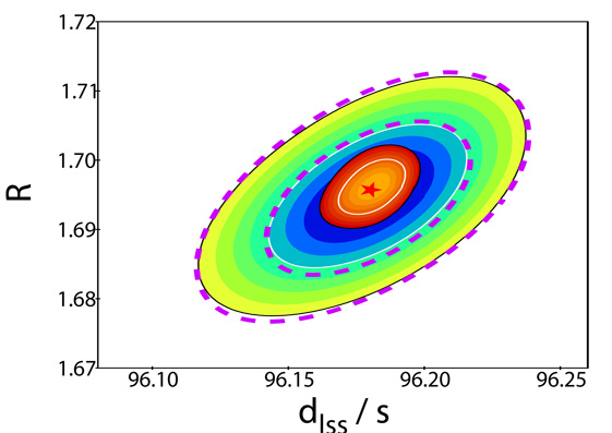Figure 11. Left panel: CMB data determines the geometric quantities of the distance to last scattering dlss and the sound horizon scale s precisely, and their ratio (the slope of the contours) - the acoustic peak angle - even more so. The contours give the 68.3% (white line) and 95.4% (black line) confidence levels for a cosmic variance limited experiment. Outer (dark blue to light green) contours use the temperature power spectrum, with dashed contours restricted to multipoles 40, while the inner (light gold to dark red) contours include the E-mode polarization and TE cross-spectrum. Right panel: Similar contours for the shift parameter R = (m h2)1/2 dlss and acoustic peak scale.

The tightly constrained geometric information means that certain combinations of cosmological parameters are well determined, but this can actually be a pitfall if one is not careful in interpretation. Under certain circumstances, one such parameter is the value of the dark energy equation of state at a particular redshift, w_* = w(z 0.4), related to a so-called pivot redshift. If CMB data is consistent with a cosmological constant universe, CDM, then this forces w_* -1. However, this does not mean that dark energy is the cosmological constant - that is merely a mirage as a wide variety of dynamical models would be forced to give the same result. See Section 5.2 for further discussion.

3.4. Baryon acoustic oscillations

The sound horizon imprinted in the density oscillations of the photon-baryon fluid, showing up as acoustic peaks and valleys in the CMB temperature power spectrum, also appears in the large scale spatial distribution of baryons. Since galaxies, galaxy clusters, and other objects containing baryons can be observed at various redshifts, measurements of the angular scale defined by the standard ruler of the sound horizon provide a distance-redshift probe. Table 1 compares the acoustic oscillations in baryons and photons.

Table 1. Comparison of signals from perturbations in the prerecombination coupled baryon-photon fluid.

	Photons	Baryons
Effect	CMB acoustic peaks	Baryon acoustic oscillations
Scale	1°	100 h-1 Mpc comoving
Base amplitude	5× 10-5	10-1
Oscillation amplitude	(1)	5%
Detection	1015/hand/sec	indirect: light from < 1010 galaxies

For spatial density patterns corresponding to baryon acoustic oscillations (BAO) transverse to the line of sight, this is an angular distance relation while radially, along the line of sight, this is a proper distance interval, corresponding in the limit of small interval to the inverse Hubble parameter since dr_prop = dz / [(1 + z)H]. It is important to remember that the quantities measured are actually distance ratios, i.e. = d_a / s and = sH. These give different dependencies on the cosmological parameters than SN distances, as rather than being ratios relative to low redshift distances they are ratios relative to the high redshift universe (see Section 3.1 and Figures 7 - 8).

The BAO scale was first measured with moderate statistical significance in 2005 with Sloan Digital Sky Survey data [49, 50, 51] and 2dF survey data [52]. Current precision is 3.6% on the angular distance measurement at z = 0.35 and 6.5% at z = 0.5. Comparing the z = 0.35 SDSS result with the 2dF result at z = 0.2 reveals some tension [53], likely between the data sets [54] rather than from major deviation from the CDM model. Note that the quantities quoted to date are not individual reduced distances but rather a roughly spherically averaged quantity convolving angular distance and proper distance interval.

To obtain the proper distance interval, and hence nearly the reduced Hubble parameter, requires accurate spectroscopic information to avoid projection of modes along the line of sight. Photometric redshifts allow estimation of the reduced angular distance but even that is at reduced precision until the redshift resolution approaches spectroscopic quality [55]. Since the sound horizon scale is about 1/30 of the Hubble radius today, assembling sufficient statistics to measure accurately the subtle signal requires huge numbers of baryon markers over great volumes (10⁶-10⁹ over 1-100 Gpc³). For early papers on the cosmological use of BAO and issues regarding the interpretation of data, see [56, 57, 58, 59, 60, 61, 62, 63, 64, 65, 66].

3.5. Other methods

Many other probes of the expansion history and cosmic acceleration have been suggested, in the geometry, geometry+mass, or geometry+mass+gas categories. However many of them either lack a robust physical foundation or have yet to achieve practical demonstration of cosmological constraints. We therefore merely list some of the geometric methods with a few brief comments.

General tests of the expansion - These are in a certain sense the most fundamental and interesting. One well known test is that the CMB temperature should evolve with redshift as T ~ 1 + z. This depends on the phase space density of the radiation being conserved, following Liouville's Theorem, e.g. photons do not convert into axions or appreciably interact with other components not in equilibrium with the radiation. It also requires the expansion to be adiabatic. Measurements to date, out to z = 3, show agreement with T ~ 1 + z at modest precision, and further prospects include using the Sunyaev-Zel'dovich effect (Compton upscattering) in clusters to sample the radiation field seen by galaxy clusters at different redshifts [67].

Another test depending on Liouville conservation is the thermodynamic, or reciprocity, relation that can be phrased as a redshift scaling between angular distances and luminosity distances or "third party" angular distances between points not including the observer. Most commonly the relation is written as d_l = (1 + z)² d_a. This has a long history in cosmology, dating from the 1930s with Tolman [68], Ruse [69], and Etherington [70], through the 1970s with Weinberg [71], and a general proof in terms of the Raychaudhuri equation and the second law of thermodynamics by [72, 31]. The thermodynamic connection is basically that if two identical blackbodies sent photons to each other in a cyclic process over cosmic distances then work would be done unless the relation holds.

While the generality of these two probes as tests of the nature of the expansion itself is intriguing, if a violation were found one might be far more likely to blame uncertainties in the sources than a radical breakdown of the physics.

Epochs of the expansion - The expansion history can also be probed at certain special epochs. For example, light element abundances are sensitive to the expansion rate during primordial nucleosynthesis [73]. The CMB recombination epoch and sound horizon are influenced by deviations from matter and radiation dominated expansion [74, 75]. In the future, if we measure the abundance and mass of dark matter particles as thermal relics, we may be able to constrain the expansion rate at their freezeout epoch near perhaps 1 TeV (z = 10¹⁶) [76]. Such early constraints are particularly interesting in multifield or multiepoch acceleration models [77].

Gamma ray bursts - As sources detectable to high redshift and insensitive to dust extinction, some hope existed that gamma ray bursts could serve as standardized candles to high redshift (but see Section 3.6 and Figure 12 regarding the limited leverage of high redshift). However, while SN have an intrinsic flux dispersion of less than 50% that one calibrates down to 15% scatter, GRBs start with an isotropic-equivalent energy dispersion of a factor 1000, making any calibration much more challenging. Standardization relations were often ill defined and sensitive to environment [78] and with better data it is now realized that much of the correlation arose from experimental selection effects [79].

Gravitational wave sources - The intrinsic amplitude of clean systems like inspiraling black hole binaries can be predicted from observations of the gravitational waveform, giving a standard siren to compare to detected gravitational wave amplitude, thus providing a distance [80, 81]. No such observations have yet been achieved. Obtaining the redshift part of the distance-redshift relation depends on observing an electromagnetic counterpart.

Gravitational lensing cosmography - Deflection of light by massive objects depends on the mass distribution, the distances of source and lens from the observer, and the laws of gravity. However, cross-correlation techniques between sources at different redshifts have been proposed to reduce the need for knowing the mass distribution to extract distances [82, 83, 84]. Practical demonstration has not yet occurred, but is an exciting prospect, and gravitational lensing also serves as a growth probe (see Section 4.3).

Environment dependent methods - Techniques that intrinsically depend on not just a single source but its environment or group properties require greater understanding of many astrophysical factors. Such techniques often have not yet established a clear or robust physical motivation for the standardization essential to a distance probe. Approaches attempted include the galaxy age-redshift relation [85, 86, 87], active galactic nuclei radio jets [88], active galactic nuclei reverberation mapping [89, 90], and starburst galaxies [91].

3.6. Summary of mapping techniques

• To map the cosmological expansion accurately requires clear, robust, mature measurement techniques.

• Observations over a range of redshifts are required to break degeneracies, or equivalently rotate likelihood contours. Complementary probes do this as well.

• Systematics control can narrow contours and prevent biases in parameter estimation; see Section 5 for further analysis and discussion.

We have seen that much of the leverage for mapping the cosmic expansion is determined by the innate cosmology dependence on the parameters, and any survey design must work within this framework. One implication of this is that there is a survey depth of diminishing returns; beyond some redshift z 2 little additional leverage accrues to measuring such high redshift distances relative to low redshift distances. That is, although the lever arm is longer, the lever is weaker. For high redshift distances measured relative to the high redshift universe, the lever arm is shorter, so again improvement in constraints stalls at high redshift.

Figure 12 illustrates that once the expansion history is determined out to, say, z 1.5 (or 2/3 the age of the universe) that it is exceedingly difficult to measure geometrically more about dark energy with any significance. Even the simple question of whether the equation of state has any deviation from the cosmological constant requires percent level accuracy. Note that at high redshift the range w [-, 0] is comprehensive in that w = - means the dark energy density contributes not at all, and w > 0 would mean it upsets matter domination at high redshift (limits on this are discussed further in Section 4.1). Thus distance probes of the expansion history are driven naturally by cosmology to cover the range from z = 0 to 1.5-2.

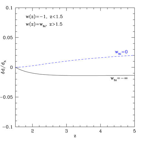Figure 12. Once the most recent two-thirds of the cosmological expansion is determined, deeper measurements of distances tied to low redshift have little further leverage. Over the physically viable range for the high redshift dark energy equation of state w [-,0], distances do not vary between models by more than 1-2%, exceedingly difficult to measure accurately at high redshift. Cosmological considerations alone indicate that covering the range out to z = 1.5-2 is the optimal strategy.