


We now address the problem of particle acceleration in clusters of galaxies. The current information on the ICM does not allow us to treat the problem as outlined above by solving the coupled kinetic equations. In what follows we make reasonable assumptions about the turbulence and the particle diffusion coefficients, and then solve the particle kinetic equation to determine N(E, t). We first consider the apparently simple scenario of acceleration of the background thermal particles. Based on some general arguments, Petrosian (2001, P01 hereafter) showed that this is not a viable mechanism. Here we carry out a more accurate calculation and show that this indeed is the case. This leads us to consider the transport and acceleration of high energy particles injected into the ICM by other processes.
3.1. Acceleration of background particles
The source particles to be accelerated are the ICM hot electrons subject to diffusion in energy space by turbulence and Coulomb collisions, acceleration by turbulence or shocks, and energy losses due to Coulomb collisions 8. We start with an ICM of kT = 8 keV, n = 10-3 cm-3 and assume a continuous injection of turbulence so that its density remains constant resulting in a time independent diffusion and acceleration rate. The results described below is from a recent paper by Petrosian & East (2007, PE07 hereafter). Following this paper we assume a simple but generic energy dependence of these coefficients. Specifically we assume a simple acceleration rate or timescale
 |
(12) |
Fig. 2 shows a few examples of these time scales along with the effective Coulomb (plus IC and synchrotron) loss times as described in Fig. 3 of Petrosian et al. 2008 - Chapter 10, this volume.
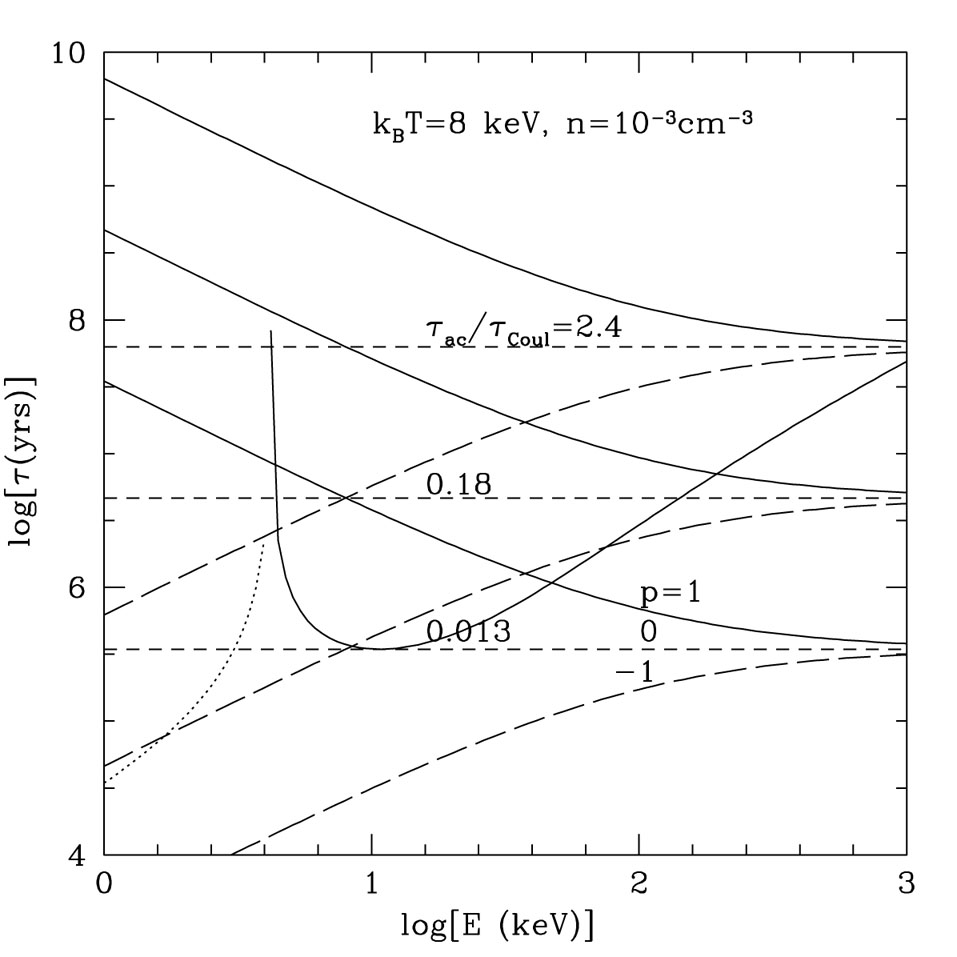 |
Figure 2.Acceleration and loss timescales
for ICM conditions based on the model described in the text. We use the
effective Coulomb loss rate given by
Petrosian
et al. 2008
- Chapter 10, this volume,
and the IC plus synchrotron losses for a CMB temperature
of TCMB = 3 K and an ICM magnetic field of
B = 1 µG. We also use
the simple acceleration scenario of Eq. 12 for
Ec = 0.2mec2 ( ~
100 keV) and for the three
specified values of p and times
|
We then use Eq. 10 to obtain the time evolution of the particle spectra.
After each time step we use the resultant spectrum to update the Coulomb
coefficients as described by
Petrosian
et al. 2008
- Chapter 10, this volume.
At each step the electron spectrum can be divided into a quasi-thermal
and a 'non-thermal' component. A best fit Maxwellian distribution to the
quasi-thermal part is obtained, and we determine a temperature and the
fraction of the thermal electrons. The remainder is labelled as the
non-thermal tail. (For more details see PE07). The left and middle panels of
Fig. 3
show two spectral evolutions for two different values of acceleration time
 0 /
Coul = 0.013 and
2.4, respectively,
and for Ec = 25 keV and p = 1. The last
spectrum in each case is for time t =
0,
corresponding to an equal energy input for all cases. The initial and final
temperatures, the fraction of particles in the quasi-thermal component
Nth, and the ratio of non-thermal to thermal energies
Rnonth are shown
for each panel. The general feature of these results is that the turbulence
causes both acceleration and heating in the sense that the spectra at low
energies resemble a thermal distribution but also have a substantial
deviation from this quasi-thermal distribution at high energies which
can be fitted by a power law over a finite energy range. The
distribution is broad and continuous, and as time progresses it becomes
broader and shifts to higher energies; the temperature increases and the
non-thermal 'tail' becomes more prominent. There is very little of a
non-thermal tail for
0 >
Coul and most of
the turbulent energy goes into heating (middle panel). Note that this
also means that for a steady state case where the rate of energy gained
from turbulence is equal to radiative energy loss rate (in this case
thermal Bremsstrahlung, with time scale >>
Coul)
there will be an insignificant non-thermal
component. There is no distinct non-thermal tail except at unreasonably high
acceleration rate (left panel). Even here there is significant heating
(almost doubling of the temperature) within a short time ( ~ 3 ×
105 yr). At such rates of acceleration most particles will
end up at energies much larger
than the initial kT and in a broad non-thermal
distribution. We have also calculated spectra for different values of
the cutoff energy Ec
and index p. As expected for larger (smaller) values of
Ec and smaller (higher) values of p the
fraction of non-thermal particles is lower (higher).
0 /
Coul = 0.013 and
2.4, respectively,
and for Ec = 25 keV and p = 1. The last
spectrum in each case is for time t =
0,
corresponding to an equal energy input for all cases. The initial and final
temperatures, the fraction of particles in the quasi-thermal component
Nth, and the ratio of non-thermal to thermal energies
Rnonth are shown
for each panel. The general feature of these results is that the turbulence
causes both acceleration and heating in the sense that the spectra at low
energies resemble a thermal distribution but also have a substantial
deviation from this quasi-thermal distribution at high energies which
can be fitted by a power law over a finite energy range. The
distribution is broad and continuous, and as time progresses it becomes
broader and shifts to higher energies; the temperature increases and the
non-thermal 'tail' becomes more prominent. There is very little of a
non-thermal tail for
0 >
Coul and most of
the turbulent energy goes into heating (middle panel). Note that this
also means that for a steady state case where the rate of energy gained
from turbulence is equal to radiative energy loss rate (in this case
thermal Bremsstrahlung, with time scale >>
Coul)
there will be an insignificant non-thermal
component. There is no distinct non-thermal tail except at unreasonably high
acceleration rate (left panel). Even here there is significant heating
(almost doubling of the temperature) within a short time ( ~ 3 ×
105 yr). At such rates of acceleration most particles will
end up at energies much larger
than the initial kT and in a broad non-thermal
distribution. We have also calculated spectra for different values of
the cutoff energy Ec
and index p. As expected for larger (smaller) values of
Ec and smaller (higher) values of p the
fraction of non-thermal particles is lower (higher).
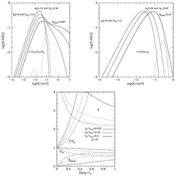 |
Figure 3. Upper left panel:
Evolution with time of electron spectra in the
presence of a constant level of turbulence that accelerates electrons
according to Eq. 12 with
|
The evolution in time of the temperature (in units of its initial
value), the
fraction of the electrons in the 'non-thermal' component, the energy ratio
Rnonth as well as an index
 = -d
lnN(E) / d lnE
for the non-thermal component are shown in the right panel of
Fig. 3. All the characteristics described above
are more clearly evident in this panel and similar ones for p =
-1 and +1. In all cases the
temperature increases by more than a factor of 2. This factor is smaller at
higher rates of acceleration. In addition, high acceleration rates produce
flatter non-thermal tails (smaller
) and a larger fraction of
non-thermal particles (smaller Nth) and energy
(Rnonth).
= -d
lnN(E) / d lnE
for the non-thermal component are shown in the right panel of
Fig. 3. All the characteristics described above
are more clearly evident in this panel and similar ones for p =
-1 and +1. In all cases the
temperature increases by more than a factor of 2. This factor is smaller at
higher rates of acceleration. In addition, high acceleration rates produce
flatter non-thermal tails (smaller
) and a larger fraction of
non-thermal particles (smaller Nth) and energy
(Rnonth).
It should be noted that the general aspects of the above behaviour are dictated by the Coulomb collisions and are fairly insensitive to the details of the acceleration mechanism which can affect the spectral evolution somewhat quantitatively but not its qualitative aspects. At low acceleration rates one gets mainly heating and at high acceleration rate a prominent non-thermal tail is present but there is also substantial heating within one acceleration timescale which for such cases is very short. Clearly in a steady state situation there will be an insignificant non-thermal component. These findings support qualitatively findings by P01 and do not support the presence of distinct non-thermal tails advocated by Blasi (2000) and Dogiel et al. (2007), but agree qualitatively with the more rigorous analysis of Wolfe & Melia (2006). For further results, discussions and comparison with earlier works see PE07.
We therefore conclude that the acceleration of background electrons stochastically or otherwise and non-thermal bremsstrahlung are not a viable mechanism for production of non-thermal hard X-ray excesses observed in some clusters of galaxies.
3.2. Acceleration of injected particles
The natural way to overcome the above difficulties is to assume that the radio and the hard X-ray radiation are produced by relativistic electrons injected in the ICM, the first via synchrotron and the second via the inverse Compton scattering of CMB photons. The energy loss rate of relativistic electrons can be approximated by (see P01)
 |
(13) |
where
 |
(14) |
are twice the loss time and the energy where the total loss curve
reaches its maximum 9
(see Fig. 4). Here
r0 = e2 / (me
c2 ) = 2.82 × 10⁻¹³ cm is the
classical electron radius, uph (due to the CMB) and
B2 / 8 are
photon (primarily CMB) and magnetic field energy densities. For the ICM
B ~ µG, n = 10-3 cm-3
and the Coulomb logarithm
ln
are
photon (primarily CMB) and magnetic field energy densities. For the ICM
B ~ µG, n = 10-3 cm-3
and the Coulomb logarithm
ln = 40
so that loss =
6.3 × 10⁹ yr and
Ep = 235 me c2.
= 40
so that loss =
6.3 × 10⁹ yr and
Ep = 235 me c2.
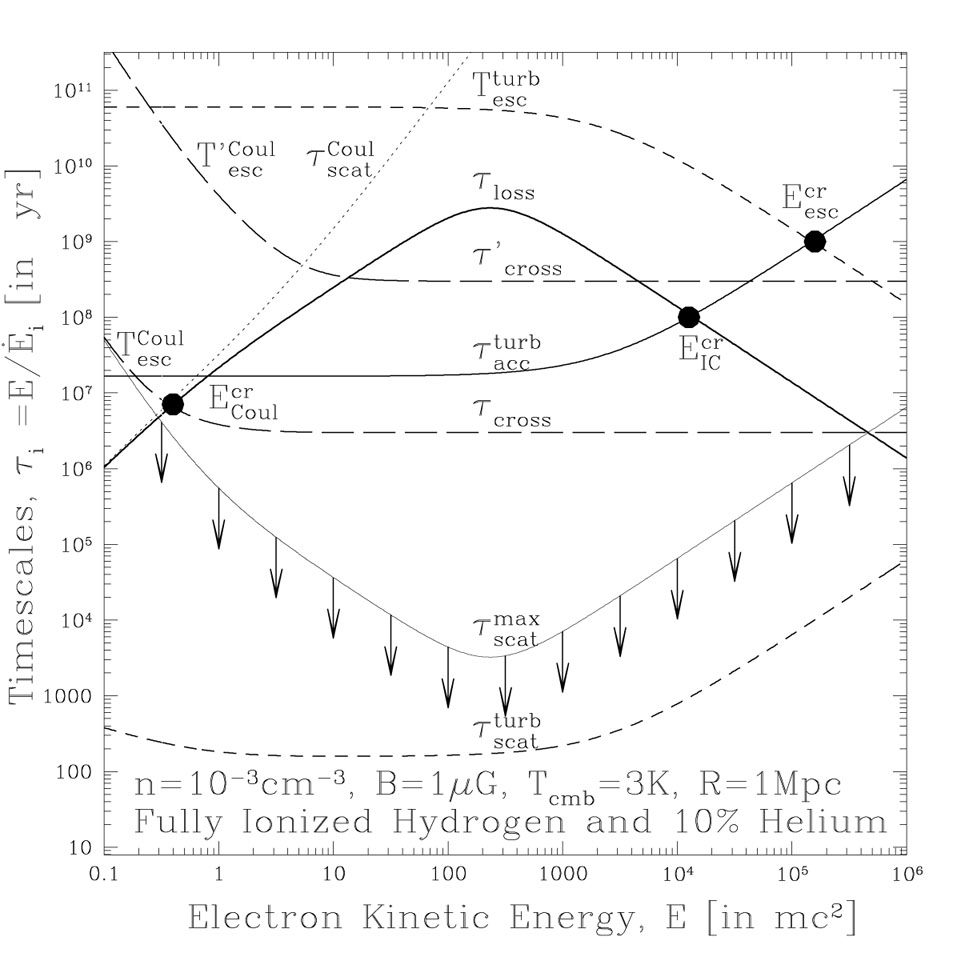 |
Figure 4. Comparison of the energy
dependence of the total loss time (radiative plus Coulomb; thick solid
line) with timescales for scattering
|
The electrons are scattered and gain energy if there is some turbulence
in the ICM. The turbulence should be such that it resonates with the
injected relativistic electrons and not the background thermal
nonrelativistic electrons for the reasons described in the previous
section. Relativistic electrons will
interact mainly with low wavevector waves in the inertial range where
W(k)  k-q with the index q ~ 5/3 or 3/2 for a
Kolmogorov or
Kraichnan cascade. There will be little interaction with nonrelativistic
background electrons if the turbulence spectrum is cut off above some
maximum wave vector kmax whose value depends on
viscosity and magnetic field. The coefficients of the transport equation
(Eq. 10) can then be approximated by
k-q with the index q ~ 5/3 or 3/2 for a
Kolmogorov or
Kraichnan cascade. There will be little interaction with nonrelativistic
background electrons if the turbulence spectrum is cut off above some
maximum wave vector kmax whose value depends on
viscosity and magnetic field. The coefficients of the transport equation
(Eq. 10) can then be approximated by
 |
(15) |
For a stochastic acceleration model at relativistic energies a =
2, but if in
addition to scattering by PWT there are other agents of acceleration (e.g.
shocks) then the coefficient a will be larger than 2. In this
model the escape time is determined by the crossing time
Tcross ~ R/c and the scattering time
scat ~
Dµµ-1. We can then write
Tesc ~
Tcross(1 + Tcross /
scat).
Some examples of these are shown in Fig. 4.
However, the escape time is also affected by
the geometry of the magnetic field (e.g. the degree of its
entanglement). For this reason we have kept the form of the escape time
to be more general. In addition to these relations we also need the
spectrum and rate of injection to
obtain the spectrum of radiating electrons. Clearly there are several
possibilities. We divided it into two categories: steady state
and time dependent. In each case we first consider only the
effects of losses, which means
 = 0 in the above expressions,
and then the effects of both acceleration and losses.
= 0 in the above expressions,
and then the effects of both acceleration and losses.
By steady state we mean variation timescales of order or larger than the
Hubble time which is also longer than the maximum loss time
loss / 2. Given
a particle injection rate
 =
0
f(E) (with
=
0
f(E) (with
 f(E)dE = 1) steady
state is possible if
f(E)dE = 1) steady
state is possible if
 esc =
0 /
N(E)E-s dE.
esc =
0 /
N(E)E-s dE.
In the absence of acceleration
( = 0) Eq. 10 can be solved
analytically. For the examples of escape times given in
Fig. 4
(Tesc >
loss) one gets
the simple cooling spectra N =
(
loss /
Ep)
e f(E)dE
/ (1 + (E / Ep)2),
which gives a spectral index break at Ep from index
p0 - 1 below to
p0 + 1 above Ep, for an injected
power law f(E)
E-p0. For
p0 = 2 this will give a high energy power law in rough
agreement with the
observations but with two caveats. The first is that the spectrum of the
injected particles must be cutoff below E ~ 100
mec2 to avoid
excessive heating and the second is that this scenario cannot produce the
broken power law or exponential cutoff we need to explain the radio
spectrum of Coma (see Fig. 6 and the discussion in
Petrosian
et al. 2008
- Chapter 10, this volume). A break is possible only if the escape time
is shorter than 0
in which case the solution of the kinetic equation for a power law
injected spectrum (p0 > 1 and s > -1)
leads to the broken power law
f(E)dE
/ (1 + (E / Ep)2),
which gives a spectral index break at Ep from index
p0 - 1 below to
p0 + 1 above Ep, for an injected
power law f(E)
E-p0. For
p0 = 2 this will give a high energy power law in rough
agreement with the
observations but with two caveats. The first is that the spectrum of the
injected particles must be cutoff below E ~ 100
mec2 to avoid
excessive heating and the second is that this scenario cannot produce the
broken power law or exponential cutoff we need to explain the radio
spectrum of Coma (see Fig. 6 and the discussion in
Petrosian
et al. 2008
- Chapter 10, this volume). A break is possible only if the escape time
is shorter than 0
in which case the solution of the kinetic equation for a power law
injected spectrum (p0 > 1 and s > -1)
leads to the broken power law
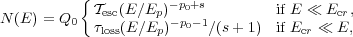 |
(16) |
where Ecr = Ep((s + 1)
(esc /
loss)-1/(s+1). Thus, for
p0 ~ 3 and s = 0 and Tesc
 0.02loss we
obtain a spectrum with a break at
Ecr ~ 104, in agreement with the
radio data
(Rephaeli
1979
model). However, this also means that a large fraction of the
E<Ep electrons escape
from the ICM, or more accurately from the turbulent confining region,
with a flux of Fesc(E)
N(E) /
Tesc(E). Such a short escape time
means a scattering time which is only ten times shorter than the
crossing time and a mean free path of about ~ 0.1R ~ 100
kpc. This is in disagreement
with the Faraday rotation observations which imply a tangled magnetic field
equivalent to a ten times smaller mean free path. The case for a long escape
time was first put forth by
Jaffe (1977).
0.02loss we
obtain a spectrum with a break at
Ecr ~ 104, in agreement with the
radio data
(Rephaeli
1979
model). However, this also means that a large fraction of the
E<Ep electrons escape
from the ICM, or more accurately from the turbulent confining region,
with a flux of Fesc(E)
N(E) /
Tesc(E). Such a short escape time
means a scattering time which is only ten times shorter than the
crossing time and a mean free path of about ~ 0.1R ~ 100
kpc. This is in disagreement
with the Faraday rotation observations which imply a tangled magnetic field
equivalent to a ten times smaller mean free path. The case for a long escape
time was first put forth by
Jaffe (1977).
Thus it appears that in addition to injection of relativistic electrons
we also need a steady presence or injection of PWT to further scatter
and accelerate the electrons. The final spectrum of electrons will
depend on the acceleration rate and its energy dependence. In general,
when the acceleration is dominant one expects a power law
spectrum. Spectral breaks appear at critical energies when this rate
becomes equal to and smaller than other rates such as the loss or escape
rates (see Fig. 4). In the energy range
where the losses can be ignored electrons injected at energy
E0(f(E) =
(E -
E0)) one expects
a power law above (and below, which we are not interested in) this
energy. In the realistic case of long Tesc (and/or
when the direct acceleration rate is larger than the rate of stochastic
acceleration (i.e. a >> 1) then spectral index of the
electrons will be equal to -q + 1 requiring a turbulence spectral
index of q = 4 which is much larger than expected values of 5/3 or
3/2 (see
Park &
Petrosian 1995).
This spectrum will become steeper (usually cut off
exponentially) above the energy where the loss time becomes equal to the
acceleration time
ac = E /
A(E)
or at Ecr = (Ep a
loss)1/(3 -
q). Steeper
spectra below this energy are possible only for shorter
Tesc. The left panel of
Fig. 5 shows the dependence of the spectra on
Tesc for q = 2 and s = 0 (acceleration and
escape times independent of E). The spectral index just above
E0 is p = (9/4 +
2ac /
Tesc)1/2 - 1.5. In the
limit when Tesc
 the distribution
approaches a relativistic Maxwellian distribution N
E2e - E / Ecr. For
a cut-off energy Ecr ~ 104 this
requires an acceleration time of ~ 108 yr and for a spectral
index of p=3 below this energy we need Tesc ~
ac/18 ~ 5 ×
106 yr which is
comparable to the unhindered crossing time. This is too short. As shown
in Fig. 4 any scattering mean free path
(or magnetic field variation scale) less than the cluster size will
automatically give a longer escape time and a flatter than required
spectrum. For further detail on all aspects of this case see
Park &
Petrosian (1995),
P01 and
Liu et
al. (2006).
the distribution
approaches a relativistic Maxwellian distribution N
E2e - E / Ecr. For
a cut-off energy Ecr ~ 104 this
requires an acceleration time of ~ 108 yr and for a spectral
index of p=3 below this energy we need Tesc ~
ac/18 ~ 5 ×
106 yr which is
comparable to the unhindered crossing time. This is too short. As shown
in Fig. 4 any scattering mean free path
(or magnetic field variation scale) less than the cluster size will
automatically give a longer escape time and a flatter than required
spectrum. For further detail on all aspects of this case see
Park &
Petrosian (1995),
P01 and
Liu et
al. (2006).
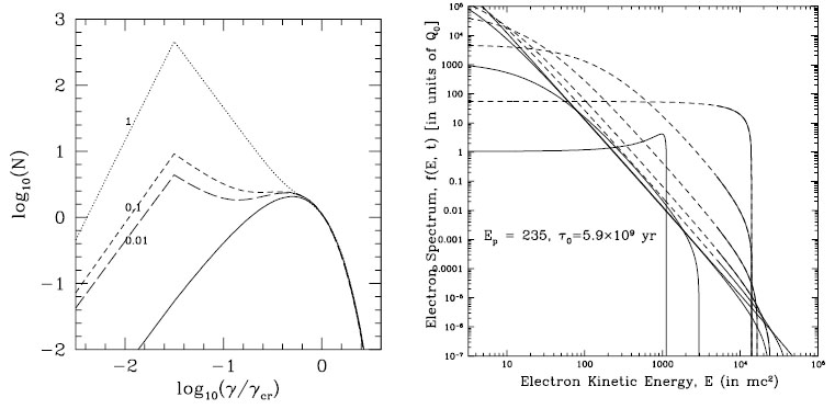 |
Figure 5. Left panel: The steady
state electron spectra injected at energy
E0 and subject to continuous acceleration by
turbulence with spectral index q = 2 for different values of the
ratio Tesc /
|
In summary there are several major difficulties with the steady state model.
We are therefore led to consider time dependent scenarios with time
variation shorter than the Hubble time. The time dependence may arise
from the episodic nature of the injection process (e.g. varying AGN
activity) and/or from episodic nature of turbulence generation process
(see e.g.
Cassano &
Brunetti 2005).
In this case we need solutions of the time dependent
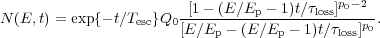
equation (Eq. 10). We start with the generic
model of a prompt single-epoch injection of electrons with
Q(E, t) = Q(E)
(t -
t0). More
complex temporal behaviour can be obtained by the convolution of the
injection time profile with the solutions described below. The results
presented below are from P01. Similar treatments of the following cases
can be found in
Brunetti et
al. (2001)
and
Brunetti
& Lazarian (2007).
It is clear that if there is no re-acceleration, electrons will lose
energy first at highest and lowest energies due to inverse Compton and
Coulomb losses, respectively. Particles will be peeled away from an
initial power law with the low and high energy cut-offs moving gradually
toward the peak energy Ep. A more varied and complex
set of spectra can be obtained if we add the effects of diffusion and
acceleration. Simple analytic solutions for the time dependent case are
possible only for special cases. Most of the complexity arises because
of the diffusion term which plays a vital role in shaping the spectrum
for a narrow injection spectrum. For some examples see
Park &
Petrosian (1996).
Here we limit our discussion to a broad initial electron spectrum in
which case
the effects of this term can be ignored until such features are
developed. Thus, if we set D(E) = 0, which is a particularly
good approximation when a >> 1, and for the purpose of
demonstration if we again consider the simple case of constant
acceleration time (q = 2 and A(E) = a
E), then the
solution of Eq. 10 gives
 |
(17) |
where 2 = 1 -
b2 / 4, b =
a
0
Ep2 =
loss /
ac and
T± = 1 ±
btan(
t / loss)
/ (2). Note that
b = 0 correspond to the case of no
acceleration described above. This solution is valid for
b2 < 4. For b2 > 4
we are dealing with an imaginary value
for so that tangents
and cosines become hyperbolic functions with
2 =
b2 / 4 - 1. For
= 0 or
b = 2 this expression reduces to
 |
(18) |
The right panel of Fig. 5 shows the evolution of
an initial power law spectrum subjected to weak acceleration (b =
2, solid lines) and a fairly
strong rate of acceleration (b = 60, dashed line). As expected with
acceleration, one can push the electron spectra to higher levels and
extend it
to higher energies. At low rates of acceleration the spectrum evolves toward
the generic case of a flat low energy part with a fairly steep cutoff above
Ep. At higher rates, and for some periods of time
comparable to
ac, the cut off
energy Ecr will be
greater than Ep and there will be a power law portion
below it. 10
As evident from this figure there are periods of time when in the relevant
energy range (thick solid lines) the spectra resemble what is needed for
describing the radio and hard X-ray observations from Coma described in Fig. 6 of
Petrosian
et al. 2008
- Chapter 10, this volume.
In summary, it appears that a steady state model has difficulties and that the most likely scenario is episodic injection of relativistic particles and/or turbulence and shocks which will re-accelerate the existing or injected relativistic electrons into a spectral shape consistent with observations. However these spectra are short lived, lasting for periods of less than a billion years.
8 In our numerical results we do include synchrotron, IC and Bremsstrahlung losses. But these have an insignificant effect in the case of nonrelativistic electrons under investigation here. Back.
9 We ignore the Bremsstrahlung loss and the weak dependence on E of Coulomb losses at nonrelativistic energies. We can also ignore the energy diffusion rate due to Coulomb scattering. Back.
10 At even later times than shown here on gets a large pile up at the cut off energy (see P01). This latter feature is of course artificial because we have neglected the diffusion term which will smooth out such features (see Brunetti & Lazarian 2007). Back.
 (long dashed lines) and escape time
Tesc ~
(long dashed lines) and escape time
Tesc ~