2. REVERBERATION MAPPING BASICS

Simply put, the idea behind reverberation mapping is to learn about the structure and kinematics of the BLR by observing the detailed response of the broad emission lines to changes in the continuum. The basic assumptions needed are few and straightforward, and can largely be justified after the fact:

1. The continuum originates in a single central source. The size of the accretion disk in a typical bright Seyfert galaxy is expected to be of order 10¹³ - 10¹⁴ cm, or about a factor of 100 or so smaller than the BLR turns out to be. It is worth noting that we do not necessarily have to assume that the continuum is emitted isotropically.

2. Light-travel time _LT = r / c is the most important time scale. The other potentially important time scales include:
   • The recombination time scale _rec = (n_{e B})^-1, which is the time for emission-line gas to re-establish photoionization equilibrium in response to a change in the continuum brightness. For typical BLR densities, n_e 10¹⁰ cm^-3, _rec 0.1 hr, i.e., virtually instantaneous relative to the light-travel timescales of days to weeks for luminous Seyfert galaxies.

   • The dynamical time scale for the BLR gas, _dyn r / V. For typical luminous Seyferts, this works out to be of order 3 - 5 years. Reverberation experiments must be kept short relative to the dynamical timescale to avoid smearing the light travel-time effects.

3. There is a simple, though not necessarily linear, relationship between the observed continuum and the ionizing continuum. In particular, the observed continuum must vary in phase with the ionizing continuum, which is what is driving the line variations. This is probably the most fragile of these assumptions since there is some evidence that long-wavelength continuum variations follow those at shorter wavelengths, but the timescales involved are still significantly shorter than the timescales for emission-line response.

Given these assumptions, a linearized response model can be written as

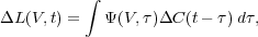(2)

where C(t) is the continuum light curve relative to its mean value , i.e., C(t) = C(t) - , and, L(V, t) is the emission-line light curve as a function of line-of-sight Doppler velocity V relative to its mean value (V). The function (V, ) is the "velocity-delay map," i.e., the BLR responsivity mapped into line-of-sight velocity/time-delay space. It is also sometimes referred to as the "transfer function" and eq. (1) is called the transfer equation. Inspection of this formula shows that the velocity-delay map is essentially the observed response to a delta-function continuum outburst. This makes it easy to construct model velocity-delay maps from first principles.

Consider first what an observer at the central source would see in response to a delta-function (instantaneous) outburst. Photons from the outburst will travel out to some distance r where they will be intercepted and absorbed by BLR clouds and produce emission-line photons in response. Some of the emission-line photons will travel back to the central source, reaching it after a time delay = 2r / c. Thus a spherical surface at distance r defines an "isodelay surface" since all emission-line photons produced on this surface are observed to have the same time delay relative to the continuum outburst. For an observer at any other location, the isodelay surface would be the locus of points for which the travel from the common initial point (the continuum source) to the observer is constant. It is obvious that such a locus is an ellipsoid. When the observer is moved to infinity, the isodelay surface becomes a paraboloid. We show a typical isodelay surface for this geometry in the top panel of Figure 1.

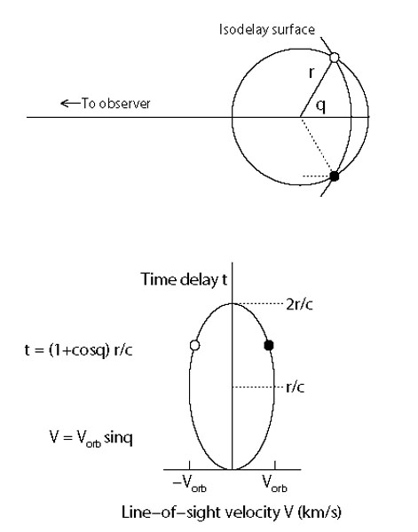Figure 1. Upper diagram: In this simple, illustrative model, the line-emitting clouds are taken to be on a circular orbit of radius r around the central black hole. The observer is to the left. In response to an instantaneous continuum outburst, the clouds seen by the distant observer at a time delay after detection of the continuum outburst will be those that lie along an "isodelay surface," for which the time delay relative to the continuum signal will be = (1 + cos)r / c, the length of the dotted path shown. Lower diagram: The circular orbit is mapped into the line-of-sight velocity/time-delay plane.

We can now construct a simple velocity delay map. Consider the trivial case of BLR that is comprised of an edge-on (inclination 90°) ring of clouds in a circular Keplerian orbit, as shown on the top panel of Figure 1. In the lower panel of Figure 1, we map the points from polar coordinates in configuration space to points in velocity-time delay space. Points (r, ) in configuration space map into line-of-sight velocity/time-delay space (V, ) according to V = -V_orb sin, where V_orb is the orbital speed, and = (1 + cos)r / c. Inspection of Figure 1 shows that a circular Keplerian orbit projects to an ellipse in velocity-time delay space. Generalization to radially extended geometries is simple: a disk is a system of rings of different radii and a spherical shell is a system of rings of different inclinations. Figure 2 shows a system of circular Keplerian orbits, i.e., V_orb(r) r^-1/2, and how these project into velocity-delay space. A key feature of Keplerian systems is the "taper" in the velocity-delay map with increasing time delay.

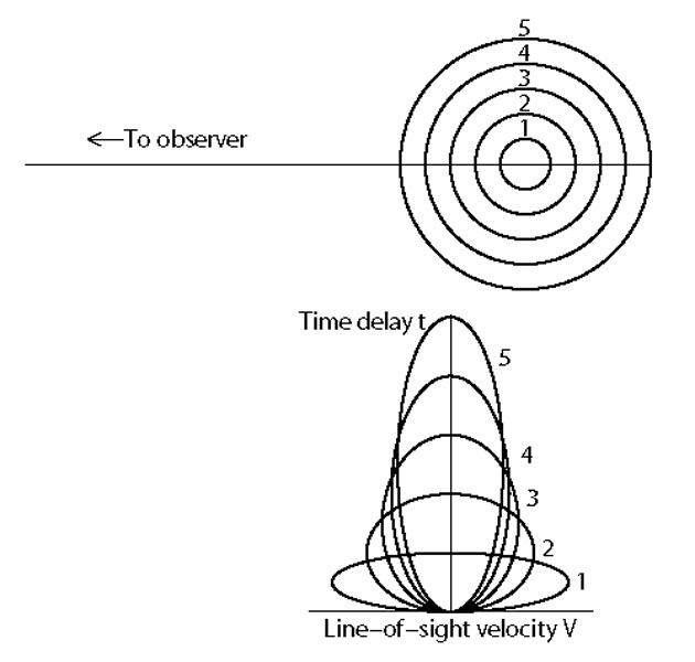Figure 2. This diagram is similar to Figure 1. Here we show how circular Keplerian orbits of different radii map into the velocity-time delay plane. Inner orbits have a larger velocity range (V r-1/2) and shorter range of time delay (max = 2r / c), resulting in tapering of the map in velocity with increasing time delay, a general feature of gravitationally dominated systems.

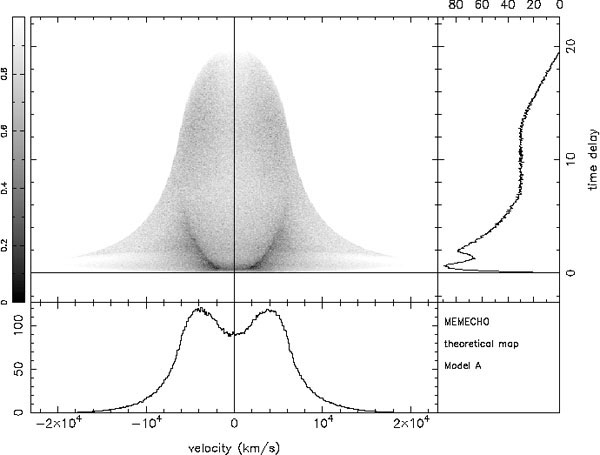
In Figure 3, we show two complete velocity-delay maps for radially extended systems, in one case a Keplerian disk and in the other a spherical system of clouds in circular Keplerian orbits of random inclination. In both examples, the velocity-delay map is shown in the upper left panel in greyscale. The lower left panel shows the result of integrating the velocity-delay map over time delay, thus yielding the emission-line profile for the system. The upper right panel shows the result of integrating over velocity, yielding the total time response of the line; this is referred to as the "delay map" or the "one-dimensional transfer function." Inspection of Figure 3 shows that these two velocity-delay maps are superficially similar; both show clearly the tapering with time delay that is characteristic of Keplerian systems and have double-peaked line profiles. However, it is also clear that they can be easily distinguished from one another. This, of course, is the key: the goal of reverberation mapping is to use the observables, namely the continuum light curve C(t) and the emission-line light curve L(V, t) and invert eq. (2) to recover the velocity-delay map (V, ). Equation (2) represents a fairly common type of problem that arises in many applications in physics and engineering. Indeed, the velocity-delay map is the Green's function for the system. Solution of eq. (2) by Fourier transforms immediately suggests itself, but real reverberation data are far too sparsely sampled and usually too noisy to this method to be effective. Other methods have to be employed, such as reconstruction by the maximum entropy method (Horne 1994). Unfortunately, even the best reverberation data obtained to date have not been up to the task of yielding a high-fidelity velocity-delay map. Existing velocity-delay maps are noisy and ambiguous. Figure 4 shows the result of an attempt to recover a velocity-delay map for the C IV - He II spectral region in NGC 4151 (Ulrich & Horne 1996). The Keplerian taper of the map is seen, but other possible structure is only hinted at, as it is in other attempt to recover a velocity-delay map from real data (e.g., Wanders et al. 1995; Done & Krolik 1996; Kollatschny 2003). It must be pointed out, however, that no case to date has recovery of the velocity-delay map been a design goal for an experiment. Previous reverberation-mapping experiments have had the more modest goal of recovering only the mean response time of emission lines, from which one can still draw considerable information. By integrating eq. (2) over velocity and then convolving it with the continuum light curve, we find that under reasonable conditions, cross-correlation of the continuum and emission-line light curves yields the mean response time, or "lag," for the emission lines.

Figure 3. Theoretical velocity-delay maps (V,) shown in greyscale for a spherical distribution of line-emitting clouds in circular Keplerian orbits of random inclination (left) and an inclined Keplerian disk of line-emitting clouds (right). Projections in velocity and time-delay show the line profile (below) and delay map (right). From Horne et al. (2004).

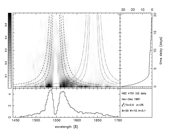Figure 4. A velocity - delay map for the C IV - He II region in NGC 4151, based on data obtained with the International Ultraviolet Explorer. From Ulrich & Horne (1996).