Annu. Rev. Astron. Astrophys. 2004. 42: 211-273 Copyright © 2004 by Annual Reviews. All rights reserved

5. SIMULATIONS OF INTERSTELLAR TURBULENCE

5.1. Introduction

Numerical simulations of the hydrodynamical or MHD equations provide the only means by which we can actually "observe" interstellar turbulence in action, although what we see depends on the physical processes included, whether and how external forcing is applied, the dimensionality of the simulations, the imposed initial and boundary conditions, the discretization technique, and the spatial resolution. The first simulations of what can now be seen as ISM turbulence go back over 20 years (Bania & Lyon 1980), but it is only within the past 5 to 10 years that the field has matured enough to concentrate on the inherently turbulent aspects of the problem.

The first simulations of nonmagnetic and nonself-gravitating supersonic turbulence at relatively high resolution were by Passot, Pouquet & Woodward (1988). Higher resolution studies of such transonic turbulence are given by Porter et al. (1999) and Porter, Pouquet & Woodward (2002). Their models are dominated by filaments in both vorticity (Figure 3) and divergence of the velocity field, and the filaments cluster into larger filaments and sheet-like structures in the compressible part of the flow, forming sheets and spirals in the vorticity field (Porter et al. 2002). Transonic nonself-gravitating models like this may illustrate the morphology of diffuse clouds and small molecular clouds when magnetic and gravitational forces are not important. They are also able to isolate the effects of moderate compressibility from other phenomena.

The first nonmagnetic simulations to include gravity were by Leorat et al. (1990) on a 128² grid, and the first nongravitating compressible simulations to include magnetic fields in an ISM context were by Yue et al. (1993) on a 20² grid. Over the next decade, these works were greatly expanded to include many aspects of the ISM, such as magnetic and gravitational forces, realistic heating and cooling, stellar energy injection and galactic shear. The first efforts in this direction were by Chiang & Prendergast (1985) and Chiang & Bregman (1988), who modeled star-formation feedback in a 2D ISM, and by Passot, Vázquez-Semadeni & Pouquet (1995), Vázquez-Semadeni, Passot & Pouquet (1995), and Vázquez-Semadeni, Passot & Pouquet (1996), who emphasized the importance of cooling and the nature of turbulent forcing, and explored the relation between magnetism and the star-formation rate. These were the first simulations to include magnetic fields, self-gravity, heating and cooling, and Coriolis forces, and were meant to represent the relatively large-scale ( ~ 1 kpc) diffuse neutral ISM. By the late 1990s, 3D MHD simulations of isothermal molecular clouds without self-gravity were performed by several groups (e.g., Mac Low et al. 1998; Stone, Ostriker & Gammie 1998; Mac Low 1999; Padoan & Nordlund 1999), and detailed comparisons with observations were made by Padoan, Jones & Nordlund (1997) and Padoan et al. (1998, 1999). Some problems with isothermal simulations are summarized in Section 4.5.

These models and others mentioned below are important steps toward understanding the complex interactions that occur in the ISM, and they provide useful statistical comparisons with observations. However, like all turbulence simulations, they have a fundamental limitation from the lack of dynamic range over the full ISM Reynolds number, Re. The number of degrees of freedom for 3D incompressible turbulence scales like Re^9/4, meaning that a simulation at Re = 10⁶ would require a resolution of 10⁵ zones per dimension, far beyond the reach of present-day approaches (but see the lattice Boltzmann method of Chen et al. 2003). Generalizing to compressible self-gravitating MHD with physically consistent driving agents and an equation of state makes the proposition even more implausible. One possibility for molecular clouds with low ionization fraction is that the energy dissipation scale is set by ambipolar diffusion and not viscosity (Klessen, Heitsch & Mac Low 2000). Then the effective Reynolds number might be (Zweibel & Brandenburg 1997)

(18)

where L is the large scale of interest, M_A the Alfvén Mach number, x the ionization fraction, n the particle density, and B the magnetic field strength. In this case the available resolution of numerical simulations would be adequate for dense molecular clouds. However this argument neglects the possibility that ambipolar diffusion acts on small scales to produce even finer structure (Brandenburg & Zweibel 1994; Tagger, Falgarone & Shukurov 1995; Balsara, Crutcher & Pouquet 2001), and it only applies in well-shielded molecular clouds, not in the general ISM.

An example of the importance of resolution for turbulence studies is the test of whether the energy flux through the inertial range is constant. This is the basis for Kolmogorov's model of incompressible turbulence, and it has only recently been verified in 2048³ simulations on the Earth Simulator (Kaneda et al. 2003). Higher resolution (4096³) simulations also find a constant energy flux, but suggest there may be a significant small departure from Kolmogorov's predicted energy spectrum (Kaneda et al. 2003). Another example is the emergence of new phenomena at very large Re, such as the transition in the power-law scaling of the flatness factor, or kurtosis, of the velocity derivative pdf observed for incompressible turbulence by Tabeling & Willaime (2002) at Taylor scale Reynolds numbers Re larger than attainable by current simulations. For compressible turbulence in the cold ISM, Adaptive Mesh Refinement simulations with effective resolution as large as 10³ × 10³ × 10⁴ have not converged yet either: a twofold increase in resolution yielded an increase in maximum density and a decrease in minimum temperature by factors greater than five (de Avillez & Breitschwerdt 2003).

Simulations at imperfect resolution can still reveal much of the underlying physics as long as the range of scales resolved is large enough that the intricate spatial fluid distortions resulting from nonlinear interactions are expressed. Resolving the inertial range for incompressible turbulence requires a resolution equivalent to more than ~ 500 zones in each direction (perhaps significantly more; Pouquet, Rosenberg, & Clyne 2003) - something that is now commonly available in 3D and easily obtained for smaller dimensions. With adequate resolution, simulations reveal geometrical and topological properties, whereas theories using statistical closure assumptions wash out the phase information. Simulations also allow many more opportunities for comparison with observations than do phenomenological or statistical models.

Here we give a brief summary of what seem to be the most important accomplishments of ISM turbulence simulations and the questions that remain unanswered. Details of numerical techniques and their associated problems are not discussed here. For example, the use of periodic boundary conditions in solving the Poisson equation introduces artificial tidal forces that can be important away from the density maxima (Gammie et al. 2003). The use of hyperviscosity, sensitivity to assumed initial conditions, differences between simulations using different numerical techniques, the violation of the Jeans condition found by Bate & Burkert (1997) and Truelove et al. (1997) in some self-gravitating simulations, and the assumption of isothermality in some simulations, are also not addressed. Systematic effects resulting from varying the parameters (especially the mean magnetic field) are also omitted (see Ostriker et al. 2001, Lee et al. 2003). Readers are referred to reviews of some of these problems and more detailed discussions of statistical properties in Vázquez-Semadeni et al. (2000), Ballesteros-Paredes (2003), Mac Low (2003), Nordlund & Padoan (2003), Ostriker (2003), and Mac Low & Klessen (2004).

5.2. Scaling Relations

Probably no result has generated more research on ISM turbulence than Larson's (1981) finding that the density and velocity dispersion of molecular clouds scale with the size of the the region as power laws, suggestive of scaling relations that are found in incompressible turbulence. Simulations have examined these relations in detail. The density-size relation found by Larson (1981), which implies a constant column density, may be a selection effect because a wide range of densities is present for each scale in the simulations, whereas observations tend to pick the strongest emission regions and select for a restricted range of column density (Kegel 1989; Scalo 1990; Vázquez-Semadeni, Ballesteros-Paredes & Rodriguez 1997; Ballesteros-Paredes & Mac Low 2002). However, Ostriker et al. (2001) reproduced Larson's squared dependence of the mass on size.

The linewidth-size relation is also problematic. Some studies show little correlation whereas others have a correlation dominated by scatter; power-law fits also vary depending on tracer and type of cloud (see references in Section 2). Even if there is a power-law with an exponent 0.4-0.6, the interpretation is ambiguous. It was attributed to a field of shock discontinuities by Vázquez-Semadeni et al. (1997), considering that the associated velocity discontinuities should give an energy spectrum E(k) k^-2 (Saffman 1971) and so v² k^-1, which gives v L^1/2. The problem with the shock model is that energy spectra found for supersonic simulations are not necessarily k^-2 (Boldyrev, Nordlund & Padoan 2002a; Wada et al. 2002; Vestuto et al. 2003). Also, the Kolmogorov spectrum for incompressible turbulence, E(k) k^-1.67, is not much different. Further, the proposed shocks themselves have not been observed directly in real clouds. Nevertheless, the linewidth-size relations in Ballesteros-Paredes & Mac Low (2002) and Kim et al. (2001) were not just virialized motions as these simulations did not include self-gravity; it is not clear whether self-gravity is required to get observed absolute scale. Kudoh & Basu (2003) obtained the Larson relations in numerical simulations of self-gravitating clouds with internal energy from magnetic waves. Other simulation studies of this relation are in Ostriker et al. (2001) and Ballesteros-Paredes & Mac Low (2002).

One problem with the linewidth-size observations is that it is impossible to identify physically coherent condensations using only radial velocities and sky coordinates of position. This was first pointed out by Burton (1971) and Adler & Roberts (1992) in connection with velocity crowding along galactic spiral arms, and then recognized for interstellar turbulence by Lazarian & Pogosyan (2000), Pichardo et al. (2000), and Ostriker et al. (2001). Another aspect of the problem is that the physically relevant correlation may be between linewidth and density (Xie 1997, Padoan et al. 2001b), which gives v n^-0.4 to n^-0.3 for Larson-like scaling. For supersonic turbulence, a relation like this makes sense because the densest regions have been decelerated behind shock fronts, although shocks propagating in a turbulent medium can increase the velocity dispersion behind them (Rotman 1991, Andreopoulos et al. 2000), which gives the opposite effect.

Another scaling relation is between magnetic field strength and density, which appears flat at densities < 100 cm^-3 and then has an upper limit that rises as B ~ n^0.5 above that (Troland & Heiles 1986, Crutcher 1999; Bourke et al. 2001). Pre-simulation work concentrated on cloud contraction, but MHD simulations account for the power index and scatter without monotonic contraction. Examples include 2D models for the diffuse ISM with self-gravity, cooling, and H II region expansion (Passot et al. 1995), isothermal 3D models with and without gravity forced with Fourier modes (Padoan & Nordlund 1999, Ostriker et al. 2001, Li et al. 2003), and 3D simulations with supernovae (Kim et al. 2001). Turbulent ambipolar diffusion could significantly affect the relation and its scatter (Heitsch et al. 2004). Passot & Vázquez-Semadeni (2003) present a detailed analysis of the problem. Other considerations are discussed in Section 5.13.

5.3. Decay of Supersonic MHD Turbulence

A major discovery of simulations is that supersonic MHD turbulence decays in roughly a crossing time (based on the rms turbulent velocity) regardless of magnetic effects and the discreteness of energy injection (Mac Low et al. 1998; Stone, Ostriker & Gammie 1998; Mac Low 1999; Padoan & Nordlund 1999; Avila-Reese & Vázquez-Semadeni 2001; Ostriker et al. 2001). Decay is faster with cooling (Kritsuk & Norman 2002b, Pavlovski et al. 2002) because the average Mach number is larger. Pavlovski et al. fit the energy to E(t) = E₀(1 + t / t₁), for t₁ = L_inj / v_rms equal to the initial ratio of the mean energy injection scale to the rms velocity, and ~ -1.3. For isothermal compressible MHD turbulence that is either super- or sub-Alfvénic, ~ -1 (e.g., Mac Low et al. 1998). This type of decay may be dominated by the pure Alfvénic (shear) modes that have this time dependence if the compressional modes are barely coupled to the shear (see Figure 1a in Cho & Lazarian 2002b). Thus, damping is not just through the compressional modes as originally thought. Alfvén wave propagation may actually delay the energy decay (Cho & Lazarian 2003). In addition, compressible modes can propagate and diffuse freely along the magnetic field lines.

Incompressible nonmagnetic turbulence is also believed to decay as a power law with time, with an exponent between about -1.2 and -1.4. Several approaches using various assumptions about the preservation of the spectrum or the nature of the low wave number part of the initial spectrum (e.g., Saffman's invariant, Loitsianskii's invariant, closures whose results depend on the initial spectrum) give results in this same range (see summaries in Hinze 1975, Lesieur 1990, Frisch 1995, Biskamp 2003). Biskamp & Müller (1999, 2000) show that for incompressible isotropic MHD turbulence the total and kinetic energies vary as t^-1 when there is no magnetic helicity but the total energy varies as t^-1/2 with the same t^-1 kinetic energy decay when helicity is present and nearly conserved. The physical reason for the similar time dependencies in the incompressible, compressible, and MHD cases is unknown.

A closely-related result, that clouds are transient entities not confined by thermal or intercloud pressure, was found by Ballesteros-Paredes, Vázquez-Semadeni & Scalo (1999) and Elmegreen (1999). These results, along with observations of short star-formation times (Ballesteros-Paredes, Hartmann & Vázquez-Semadeni 1999; Elmegreen 2000; Hartmann et al. 2001), eliminate the old problem of how clouds could be supported for long times in the presence of supersonic turbulence (Zuckerman & Evans 1974).

The details of shock energy dissipation in 3D supersonic turbulence have been studied by Smith, Mac Low & Heitsch (2000) and Smith, Mac Low & Zuev (2000) for decaying and uniformly (Fourier) forced motions; the latter paper includes models with self-gravity. Besides the frequency distribution of shock velocities whose form is explained with a phenomenological theory, Smith et al. find that in the decaying runs the dissipation rate peaks at small Mach numbers. For example, at rms Mach number of 5, the power loss peaks around Mach 1 to 2, while at rms Mach 50 the peak is from Mach 1 to 4, decreasing with time in both cases. Most of the dissipation is from a large number of weak shocks. In uniformly forced simulations, however, the dissipation occurs in a small range of high Mach number shocks, peaking at greater than the rms value. This result emphasizes the crucial role of the driving process in controlling interstellar turbulence and line profiles. For example the smoothness of line profiles (see Section 2) may imply that cool clouds spend most of their time in the decaying mode, with only sporatic and/or spatially discrete forcing. It is notable that in both cases the magnetic field had little effect on the distribution of shock strengths or their dissipation rate. As stated by Smith, Mac Low & Heitsch (2000), magnetic pressure is not damping the shocks but helps maintain them by transferring energy from the strong magnetic waves to the shock waves.

5.4. The Density Probability Distribution

Vázquez-Semadeni (1994) suggested that the probability distribution of densities (the density pdf) is lognormal as a result of the central limit theorem applied to a multiplicative hierarchical density field. Several groups subsequently found that the pdf should exhibit an approximately lognormal distribution if the gas is isothermal (Ostriker, Gammie & Stone 1999; Klessen 2000; Ostriker et al. 2001; Li et al. 2003), with quasi-power-law tails if nonisothermal (Passot & Vázquez-Semadeni 1998; Scalo et al. 1998; Nordlund & Padoan 1999). Recent simulations of dense cluster formation (Li, Klessen & Mac Low 2003) confirm the approximately lognormal behavior for isothermal turbulence and the increasingly prominent high-density tail that appears when the equation of state is softer. Li et al. (2003) find density pdfs with negative skewness from shocks that evacuate large regions, and positive skewness from self-gravity that makes clumps. The large-scale central disk galaxy simulations by Wada & Norman (2001) find a surprisingly robust and invariant lognormal form of the density pdf (above the average density) when the density field is generated by turbulence that includes a variety of physical processes. At densities below the peak the pdf found by Wada and Norman departs significantly from a lognormal.

This important theoretical result is difficult to verify from observations of column densities alone. Gaustad & VanBuren (1993) sampled the three-dimensional density distribution for fairly low densities, ~ 1 cm^-3, using 1800 OB stars as probes of the local dust density. Their pdf resembles a lognormal but it can also be fit by a power law above the mean. Berkhuijsen (1999) measured the volume filling factor as a function of density for ionized and neutral gas and obtained a power law.

The probability distribution function for column density was studied theoretically by Padoan et al. (2000), Ostriker et al. (2001), and Vázquez-Semadeni & García (2001) using numerical simulations of isothermal MHD turbulence. For the isothermal case the spatial density distribution is log-normal, so the column density distribution is similar except for blending, which depends on the ratio of cloud depth to autocorrelation length. For a large ratio, the central limit theorem gives a Gaussian distribution of column densities and for a very large ratio the column density becomes nearly constant over the face of the cloud (Vázquez-Semadeni & García 2001).

5.5. Energy Cascades

One of the oldest ideas in turbulence theory is that energy cascades in wave number space. Molecular cloud simulations often inject energy at large scales, and this energy cascades to smaller scales where dissipation occurs. In analytical work, the transfer is usually assumed to occur locally in wave number space, i.e., between similar-sized regions (compare Section 4.12). In fact, it is not well understood why turbulence cascades in a given direction or how important nonlocal energy transfer is (see Zhou, Yeung & Brasseur 1996). Good examples of nonlocal transfers are in shocks, where large-scale flows abruptly convert kinetic energy into atomic random motions at the front, and superbubbles, where localized energy gets transferred in a single step to much larger scales. In 2D incompressible turbulence, the energy cascades to large scales regardless of where it is injected; only the mean squared vorticity (enstrophy) cascades down to the viscous scale. Recent work (Kurien, Taylor & Matsumoto 2003) even indicates that the inertial range of incompressible turbulence is a dual cascade of energy and helicity that generates a k^-5/3 energy spectrum at intermediate wave numbers but k^-4/3 at large wave numbers.

How should interstellar turbulence cascade? Energy could be fed in from rotation on the largest scales, self-gravity on intermediate scales, and individual stars or clusters on intermediate to small scales. The key concept behind a direct cascade to smaller scales is absent, i.e., that an inertial range exists in which advection alone distorts the fluid elements while conserving kinetic energy. In addition, ISM turbulence is highly compressible, so there is no quadratic invariant conserved by the advection operator; energy can transfer directly between kinetic and thermal modes.

Energy may cascade in either direction or in both simultaneously. Most simulations that observe a cascade to small scales force the turbulence over the whole computational domain and often use purely solenoidal fluctuations, which favor the direct cascade. Recently, Wada et al. (2002) showed that for 2D inner galaxy models, the energy injected by self-gravity on ~ 10 pc scales cascades to larger regions; this is probably not an artifact of the 2D geometry because the system is strongly compressible and does not have the conservation properties that give incompressible 2D turbulence an inverse cascade. Vestuto, Ostriker & Stone (2003) found an inverse cascade in MHD simulations where the forcing was not at the largest scales. Christensson, Hindmarsh & Brandenburg (2001) found inverse cascade in decaying 3D MHD turbulence with helical fields. Because the range of wave number space over which forcing by H II regions, supernovae, and superbubbles occurs is extremely broad and the energy input rate is relatively uniform, the energy flow between scales in ISM turbulence remains essentially unknown. Strong forcing over a wide range of scales could even remove intermittency effects (Biferale, Lanotte & Toschi 2003).

5.6. Compressible versus Solenoidal Motions

Any turbulent velocity field can be decomposed into a solenoidal (rotational) mode and a compressible (potential or irrotational) mode and each mode can feed the other (Sasao 1973). It is of great interest to know the relative energy in each. Intuitively it might seem that the result should scale with Mach number because at zero Mach number the flow is purely incompressible and at infinite Mach number it should be mostly compressible. Some discussion of the flow of energy between the two modes, based on the coupling of the evolution equations for the vorticity and dilatation, is given by Vázquez-Semadeni et al. (1996) and Kornreich & Scalo (2000). Bataille & Zhou (1999) and Bertoglio, Bataille & Marion (2001) used a closure method with simulations to predict that the compressible to solenoidal energy ratio should increase with the square of the rms Mach number for very small Mach numbers. However, Shivamoggi (1997) used a statistical mechanical approach and found that the advection operator should evolve toward an equipartition between compressible and vortical modes.

What do simulations have to say about this ratio? A major problem with simulations, especially at the molecular cloud level, is the use of large-scale forcing in Fourier space. This has the effect of stirring the gas in the entire computational domain simultaneously. The situation in the ISM, at least at intermediate and small scales, is likely to be different. Artificial forcing is usually solenoidal also, whereas stellar energy sources will mostly generate compressible fluctuations. Generally, in the magnetic case, the solenoidal component is maintained at finite levels by magnetic torsions but in the nonmagnetic case it can become very small (Vázquez-Semadeni, Passot & Pouquet 1996).

Nordlund & Padoan (2003) explain their solenoidal/compressional ratio of 2/1 geometrically: Interacting flows generate shear in two dimensions but compression is only normal to the intersection plane. Other simulations have solenoidal/compressional ratios ranging from less than unity (Vázquez-Semadeni et al. 1996) to 5-10, depending on Mach number (Boldyrev, Nordlund & Padoan 2002b, Porter et al. 2002 - the quantity quoted in the text of Porter et al. 2002 is E_Com / E_tot whereas the quantity plotted in their Figure 2 is E_Com / E_Vor). Most results are controlled by the degree to which the forcing is solenoidal or compressible, the initial value of their ratio (Porter et al. 2002), the rms Mach number, the magnetic field strength, and the importance of cooling (Vázquez-Semadeni et al. 1996). Vestuto, Ostriker & Stone (2003) found that the solenoidal/compressional ratio increases with higher magnetic field strength, verifying an effect present in simulations by Passot et al. (1995) and Vázquez-Semadeni et al. (1996). The unforced simulations of Kritsuk & Norman (2003) have an initially high fraction of turbulent energy in the compressible form following thermal instabilities and pancake formation, and then the energy converts into mostly solenoidal form as the turbulence decays owing to baroclinic vorticity generation from shell instabilities. The value of this ratio was unfortunately not given in papers whose simulations included supernova energy input; those should be the most realistic for the ISM.

5.7. Filamentary Structure

The prevalence of filaments in the ISM has never been adequately explained by turbulence theory, although they are obviously present in the majority of simulations. Some ISM filaments are not from turbulence but are the edges of expanding shells, cometary tails of shocked clouds, or shocked regions in spiral density waves. However, filamentary structure appears elsewhere too, even in regions without obvious pressure sources (Kulkarni & Heiles 1988, Jackson et al. 2003), and it occurs with similar morphologies in turbulence simulations. Prominent suggestions for the origin of these turbulence filaments include oblique shocks or shock intersections, expanding gas along magnetic field lines, confinement by helical magnetic fields, cooling instabilities in a flattened large-scale structure, vorticity tubes from solenoidal motions, and ambipolar diffusion.

Filamentary structure is often the result of shock interactions (Heitsch et al. 2001). Even in the simulations by Balsara, Ward-Thompson & Crutcher (2001), who emphasized the role of magnetic field alignments, filaments were still found in the converging flows. However, filamentary structures are also prevalent in low Mach number, nonmagnetic simulations (Porter, Pouquet & Woodward 2002), where solenoidal forcing keeps the compressible energy low and the shocks rare; they dominate the vorticity field of incompressible turbulence (Figure 3).

5.8. Thermal Instability and Thermal Phases

The idea that thermal instability drives ISM condensation to distinct phases (Field, Goldsmith & Habing 1969) has lost much of its appeal as a result of simulations that explicitly allow the instability to operate. Vázquez-Semadeni, Gazol & Scalo (2000) and Sánchez-Salcedo, Vázquez-Semadeni & Gazol (2002) showed how turbulence smears the bimodal density distribution expected in an ISM whose structure forms solely by thermal instability. The nonlinear development of a thermal instability in an initially quiescent medium generates turbulence that reduces the initial signature of the instability (Kritsuk & Norman 2002b). These results do not arise because of strong departures from thermal equilibrium (which is usually a good approximation away from shocks), but simply because there is so much more kinetic than thermal energy in supersonic turbulence.

Thermal pressure equilibrium of clouds is of minor importance in a turbulent ISM (Ballesteros-Paredes, Vázquez-Semadeni & Scalo 1999). A high fraction of the gas mass can be in the thermally unstable regime. In the instability model, the underheated regions in the unstable regime are slightly denser and at lower pressure than the overheated regions so they contract at the sound speed to become denser and more underheated. In a turbulent medium, however, the underheated regions are not necessarily at low pressure because they are pushed around by the surrounding flow (Gazol et al. 2001). Large unstable fractions have also been found in high resolution simulations of supernova-driven turbulence (de Avillez & Breitschwerdt 2004).

These results explain the observed large fraction of interstellar gas in the supposedly unstable regime (Dickey, Salpeter & Terzian 1977; Heiles 2001; Kanekar et al. 2003) and they explain the much broader range of observed pressures than expected in the thermal instability model Jenkins 2004), as shown by Kim, Balsara & Mac Low (2001). Neither of these features can be explained by nonturbulent thermal instability models with pressure equilibrium.

5.9. Supernova-Driven Turbulence

Numerical simulations that have sufficient dynamic range to include supernovae (Gazol-Patiño & Passot 1999; Korpi et al. 1999a, b; de Avillez 2000; de Avillez & Berry 2001; Kim, Balsara & Mac Low 2001; Wada & Norman 2001; Shukurov et al. 2004) produce a continuous distribution of physical quantities, unlike the previously prevailing paradigm of discrete ISM phases (Section 5.8). Temperatures weighted by volume segregate into quasidiscrete ranges because the time spent in each temperature range is proportional to the inverse of the derivative of the cooling function (Gerola et al. 1974). The density distribution is not bi- or multimodal, however, as in a true multiphase ISM. Thus, filling fractions of gas with various temperatures may be approximately stable over long times in a statistical sense, but these should not be interpreted as phases since no phase transition is involved. Shukurov et al. (2004) and Sarson et al. (2003) find that the filling factor of hot gas is dependent on the presence, strength, and topology of the magnetic field since a strongly ordered field confines the expanding gas produced by supernovae. In the models by Wada & Norman (1999), the hot gas is heated primarily by turbulence itself.

Comparisons between these studies are difficult because some include self-gravity (Wada & Norman 2001) and magnetic fields (Gazol-Patiño & Passot 1999) but are 2D, whereas others are 3D and either include the magnetic field with no self-gravity (Korpi et al. 1999a, Kim et al. 2001, Shukurov et al. 2004) or include neither field nor gravity (de Avillez 2000, de Avillez & Berry 2001). There are also significant differences in the adopted spatial distribution of the supernova explosions. For example, Gazol-Patiño & Passot (1999), Wada & Norman (2001), and Shukurov et al. (2004) allow the supernovae to explode only at sites where the turbulence produces local conditions conducive to star formation, whereas Kim et al. (2001) explode supernovae randomly. There are additional differences concerning how this energy is distributed in time (e.g., whether a wind is allowed before the explosion). Many of these studies concentrate on the resulting distribution of warm and hot gas, so it is difficult to see from the published results how the phenomenology of the dense gas is affected; in Shukurov et al. (2004), the cold gas is explicitly omitted.

Nevertheless, the wealth of structure found in these simulations is impressive. de Avillez (2000), de Avillez & Berry (2001), and de Avillez & Breitschwerdt (2004) modeled the 3D vertical structure in a galaxy disk at high resolution and found an amazing array of structure over 400 Myr, including a thin cold disk extruding vertical "worms" and a thick frothy disk of warm neutral gas, thin sheets representing superbubble interactions connected by tunnel-like structures, small clouds resulting from the interaction and breakup of worms and sheets, networks of hot gas, and "chimneys" rising high above the plane (see also Rosen, Bregman & Norman 1993).

The evolution of supernova remnants and superbubbles in a 3D MHD turbulent medium is substantially different than in a uniform external medium. Balsara, Benjamin & Cox (2001) showed how the induced time variations of synchrotron emission in young remnants might serve as a diagnostic for the ambient medium, and they pointed out how shock amplification of turbulent motions might be important for cosmic rays. Korpi et al. (1999b) showed that superbubble breakout from galactic disks is easier in a turbulent medium because of deformation of the expansion.

5.10. The Role of Self-Gravity in the ISM

Elmegreen (1993) suggested that dense clouds or cloud cores could form in colliding turbulent gas streams and that gravitational instabilities in the shocked regions would lead to collapse and star formation. The formation of self-gravitating condensations in converging streams was suggested before this (Hunter et al. 1986), but it was uncertain whether the compressed regions in a turbulent flow would be large enough and live long enough to collapse gravitationally before they dispersed. Ballesteros-Paredes, Vázquez-Semadeni & Scalo (1999) confirmed that density maxima in turbulent flows coincide with abrupt velocity jumps, indicating shock formation. Other simulations showed that dense regions generally form by oblique stream collisions and intersecting shocks, and that the most strongly self-gravitating of these regions have enough time to collapse significantly (see Nordlund & Padoan 2003). Accretion and core-core collisions often follow with more and more of the gas entering this gravitating state. This process may terminate in a real cloud when the resulting star formation becomes intense enough to push the remaining gas away, or when the Mach number drops below one (Section 5.11).

The ability of nongravitating turbulence to fragment the ISM or the interior of a GMC down to stellar masses and below leads to a new concept for the role of gravity in forming interstellar structure and stars (see Mac Low & Klessen 2004 for a comprehensive review). Clouds and clumps are no longer seen as the result of gravitational instabilities in a region containing a large number of Jeans masses, but simply the result of supersonic turbulence, whatever the source. On kpc scales, this turbulence may be driven by interstellar gravity through swing-amplified spiral arms, so gravity is important, but much of the cloudy structure on smaller scales, including whole GMCs and their cores and clumps, could result entirely from "turbulent fragmentation," a term that dates back to Kolesnik & Ogul'Chanskii (1990). Cloud structure also results from pressurized shell formation, spiral arm shocks, and other processes, but even in these cases, the hierarchical clumpiness inside the clouds probably arises from supersonic turbulence.

The role of gravity in determining gas structure is small when the motions are faster than the virial speed. This is the case for the diffuse ISM and the smaller H I and molecular clouds (Heyer et al. 2001), and it applies to most of the small clumps inside clouds (Loren 1989, Bertoldi & McKee 1992, Falgarone et al. 1992). Self-gravitating non-magnetic simulations by Klessen (2001) confirm that the fraction of clumps with significant self-gravity increases with mass. Many cloud properties can be matched by MHD simulations without gravity, including the statistical properties of extinction and intensity, the magnetic field strength-density correlation, the size-linewidth relation, and the absolute value and size independence of core rotation (Padoan & Nordlund 1999; Kim, Balsara & Mac Low 2001; Ostriker et al. 2001; Ballesteros-Paredes & Mac Low 2002; Nordlund & Padoan 2003). The appearance of Bonner-Ebert density profiles does not imply self-gravity either because turbulent condensations can have this property even when they are not in equilibrium (Ballesteros-Paredes, Klessen & Vázquez-Semadeni 2003). Quasihydrostatic structures are actually difficult to produce by turbulent fragmentation (Ballesteros-Paredes, Vázquez-Semadeni & Scalo 1999). Moreover, the mass functions of dense cores resemble the stellar initial mass function (IMF) in both nongravitating (see Nordlund & Padoan 2003) and gravitating (Li, Klessen & Mac Low 2003) simulations because the dense local regions that can collapse were generated by turbulent interactions, not gravitational instabilities. Self-gravity is mainly important for the dense cores of turbulent regions, whereas the large-scale structure is decoupled from these cores (Ossenkopf et al. 2001).

If turbulence is viewed as preventing global collapse, then it is not because of some "turbulent pressure." In fact the conditions required for turbulence to be represented as a pressure are quite severe (Bonazzola et al. 1992), requiring a scale separation for turbulent fluctuations (Section 4.10). Structures generated by turbulence, even if bound, can be immune to global collapse because the gravitational and turbulent energy is transferred quickly to motions of substructures on smaller and smaller scales, and the densest of these small structures does the collapsing instead of the whole cloud. Collapse of turbulence-compressed cores requires a low effective ratio of specific heats dlogP / dlog = < 2(1 - 1 / n), where n = 3,2, or 1 for spherical, planar, or filamentary compressions, so the gravitational energy change exceeds the compressional energy change (Vázquez-Semadeni, Passot & Pouquet 1996)

5.11. Formation of Star Clusters and the IMF

One of the holy grails of ISM simulations has been to follow the collapse and fragmentation of a cloud to form a stellar cluster and to calculate the resulting initial mass function of stars, a goal that has been thwarted until recently by severe resolution requirements. The first studies of this type did not include self-gravity but showed that the resulting cores would collapse if self-gravity were present, given their masses and densities (see Nordlund & Padoan 2003 and references therein). Self-gravitating models illustrate the process in detail (Bonnell et al. 1997, 2003; Klessen, Burkert & Bate 1998; Klessen & Burkert 2000; Klessen, Heitsch & Mac Low 2000), including magnetic fields (Heitsch, Mac Low & Klessen 2001; Bate, Bonnell & Bromm 2003; Li et al. 2003). Figure 5 shows a simulation result from Bonnell et al. (2003). The time sequence illustrates the collapse of nonmagnetic gas into sink-particles ("stars"), competition among these particles for gas, and the formation of disks, binaries, and complex turbulent structures.

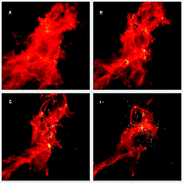Figure 5. Four time steps in an SPH hydrodynamic simulation with self-gravity and 5 × 105 fluid particles. Collapsing cores that represent stars are replaced by sink particles in the simulation and are shown here by white dots. Most stars form in a very dense gaseous core and then get ejected into the general cluster field by two-body interactions. Objects ranging in mass from brown dwarfs to ~ 30 M stars are made (from Bonnell et al. 2003.) (for slightly higher resolution, see paperI-f5.gif)

Klessen (2001) examined the mass spectrum of collapsing cores in nonmagnetic, self-gravitating turbulence simulations and found good agreement with the overall form of the stellar IMF (see observations in Chabrier 2003). It is interesting that roughly similar clump mass spectra have been found in simulations including self-gravity but neglecting magnetic fields (see also Klessen & Burkert 2001), simulations that include magnetic fields but not self-gravity (Ballesteros-Paredes & Mac Low 2002), and simulations that include both (Gammie et al. 2003). Differences do appear, but it is difficult to disentangle them from variations resulting from numerical techniques and core definitions.

Gammie et al. (2003) presented a detailed discussion of the mass spectra of gravitating and nonself-gravitating clumps in 3D self-gravitating, decaying MHD simulations. They found that the slope of the high-mass part of the spectrum becomes shallower with time, that the magnetic field strength does not affect the spectrum significantly, and that the spectrum depends on how the clumps are defined (Ballesteros-Paredes & Mac Low 2002). The dependence of the clump mass spectrum and the IMF on the equation of state was studied by Li, Klessen & Mac Low (2003). A dependence of the substellar mass function on the power spectrum of turbulence was found by Delgado-Donate, Clarke & Bate (2004).

5.12. Rotation and Binary Star Formation

The rotational properties of molecular clouds and cores have been investigated by several groups (e.g., Goldsmith & Arquilla 1985, Goodman et al. 1993, Caselli et al. 2002). Detectible gradients range mostly from 0.3 to 3 km s^-2 pc^-1. Although the average ratio of rotational to gravitational energy is small ( ~ 0.03), the nature of these gradients has been obscure.

Burkert & Bodenheimer (2000) used synthetic velocity fields with an assumed linewidth-size relation to show that even if turbulent motions are random, the dominance of large-scale modes can lead to velocity gradients that look like ordered rotation. The resulting core rotational properties as functions of size and the spread in the ratio of rotational to gravitational energies were in good agreement with observations, including the spread in binary periods, although the median angular momentum in the models was about an order of magnitude larger than in the observations. Gammie et al. (2003) studied properties of cores in 3D MHD simulations of molecular clouds and also found angular momenta larger than observed; they suggested higher resolution would eventually allow simulations to probe turbulence-produced angular momentum on the scale of binary star orbits. Fisher (2004) used a semianalytic approach to show that the distribution of binary periods was consistent with turbulence.

These results apply only to cores that are mildly subsonic. Whether the small velocity gradients detected in some larger dark clouds can be accounted for by turbulence alone remains to be seen (but see Kim, Ostriker & Stone 2003). Some gradients are probably from pressurized motions. In any case, the angular momentum problem that played a central role in most early discussions of star formation (e.g., Mouschovias 1991) is beginning to disappear. Angular momentum is still conserved in a turbulent ISM, but it gets channeled mostly into vorticity structures as turbulence distributes its energy among scales. It is unknown whether turbulence can also explain the low levels of rotation in prestellar cores (Jessop & Ward-Thompson 2001).

Turbulence simulations are approaching the scales on which binary star angular momenta are determined (Bate, Bonnell & Bromm 2002; Gammie et al. 2003). Even mild levels of turbulence during a collapse can induce multiple star formation (Klein et al. 2003; Goodwin, Whitworth & Ward-Thompson 2004).

5.13. Effects of Magnetic Fields on Interstellar Turbulence

Most MHD simulations suggest that magnetic fields have a smaller role in the ISM than previously expected. For example, they seem unable to postpone the energy dissipation in a supersonically turbulent medium (Section 5.3) and unable to prevent local gravitational collapse unless they are strong (Heitsch et al. 2001; Ostriker et al. 2001; however, see Kudoh & Basu 2003). Passot & Vázquez-Semadeni (2003) and Cho & Lazarian (2003) demonstrated that magnetic fluctuations do not act as an effective pressure at high Mach numbers because of their lack of one-to-one correspondence with density: The field acts more like a random forcing of the turbulence. What magnetic fields appear to do is reduce the core density contrast (Balsara, Crutcher & Pouquet 2001) and slow down the local collapse rate (Heitsch et al. 2001). This may not affect the overall star-formation rate much because the timescale for core formation is much longer than the core collapse itself. For turbulent fragmentation, star-formation rates should be regulated on the largest scale where the dynamical time is longest. The marginal effects of magnetic fields on the clump or core mass spectra and presumably the stellar IMF were discussed in Section 5.11. Padoan & Nordlund (1999) suggested that magnetic fields are relatively weak in molecular clouds, having energy densities less than turbulent so the motions are super-Alfvénic (see review in Nordlund & Padoan 2003).

Polarization observations show smooth magnetic fields, but this does not mean turbulence is absent (see review by Ostriker 2003). As discussed by Vázquez-Semadeni et al. (1998), cloud formation by turbulence can compress the field perpendicular to the compression direction, making it elongated in the same direction as the cloud; turbulent magnetic field-energy spectra are peaked at small wave numbers in simulations, so the field should be dominated by the largest scales, and the observed field orientations are an average on the line of sight (Heiles et al. 1993, Goodman et al. 1990). Visual polarization also probes only a small range of extinction.

Ambipolar diffusion is relatively unimportant in the overall dynamics of molecular cloud turbulence at high Mach numbers (Balsara, Crutcher & Pouquet 2001). Indeed, observations now suggest that ion-neutral drift is rapid at ~ 10⁶ cm^-3, based on comparisons of HCO+ and HCN linewidths (Houde et al. 2002). The old idea that protostellar cores form on timescales controlled by ambipolar diffusion may not apply.

Ion-neutral drift is not without consequences, however. The ambipolar diffusion heating rate in molecular cloud turbulence simulations (Padoan, Zweibel & Nordlund 2000) can be orders of magnitude larger on small scales than the background heating rate by cosmic rays, and even the volume-averaged drift heating rate can exceed the cosmic ray heating rate (Scalo 1977). Heating can be important if dynamical effects are not because there is much less thermal energy than kinetic energy in a supersonic flow. Drift heating is also more important locally because it depends on a high-order derivative of the magnetic field. Thus, turbulence can enhance ambipolar diffusion by driving structures to smaller scales (Zweibel 2002, Heitsch et al. 2004) and compressing the field (Fatuzzo & Adams 2002). Ambipolar diffusion also leads to sharp filamentary structures (Brandenburg & Zweibel 1994; Mac Low et al. 1995; Tagger, Falgarone & Shukurov 1995), rather than diffusive smoothing as once thought.

Turbulent cloud simulations (Gammie et al. 2003) also illustrate why the observed clumps and cores in molecular clouds tend to be prolate (Myers et al. 1991, Ryden 1996) with no preferred orientation relative to the field (Goodman et al. 1990). Quasistatic models with a slow contraction along field lines predicted oblate and aligned cores.

Another interesting result concerning magnetic fields is the possibility that they could control the accretion rate onto protostellar cores or larger structures. Balsara, Ward-Thompson & Crutcher (2001) found with 256³ self-gravitating MHD simulations that molecular cloud cores tend to accrete matter nonuniformly along interconnecting magnetic filaments. They cite evidence for this process in the S106 molecular cloud using ¹³CO channel maps, submillimeter maps, and polarimetry. Falgarone, Pety & Phillips (2001) found six dense filaments pointing toward the starless core L1512 extending out to about 1 pc, with evidence for the filamentary matter moving toward the core. In this case the final masses of prestellar cores could be controlled in part by the topology of the magnetic field.

Another magnetic effect is angular momentum braking, which has been discussed for decades using idealized models of clouds and fields. In a turbulent medium the magnetic field structure and its connection to density condensations is complex, and there is no guarantee that braking will occur. Vázquez-Semadeni, Passot & Pouquet (1996) and Vestuto, Ostriker & Stone (2003) show relatively more power in rotational and shear energy than compressional energy as the field strength increases, contrary to naive models of magnetic braking.

That magnetic braking does occur in a turbulent fluid with complex fields has been shown in simulations of the magnetorotational instability on a galactic scale (Kim, Ostriker & Stone 2003). The degree of braking of their largest coherent condensations may explain the low specific angular momenta inferred for molecular clouds. This is a much larger scale than star-forming cores, but the basic effect of angular momentum transfer along field lines is analogous to the cases considered in idealized collapse models by Mouschovias & Paleologou (1979) and others.

A different approach was introduced by Cho and coworkers (see Cho & Lazarian 2002a, b; Cho, Lazarian & Vishniac 2002a,b), Maron & Goldreich (2001), and Müller & Biskamp (2003) using a combination of theoretical calculations and simulations to address the properties of anisotropic Kolmogorov turbulence. They emphasized regimes that are more appropriate to the diffuse ionized ISM than dense cold regions. Several interesting and fundamental results have come from this, as reviewed in Section 4.13 and Interstellar Turbulence II.

5.14. Turbulent Rotating Galaxy Disk Simulations

Simulation codes are finally becoming sophisticated enough to model at least the central regions of differentially rotating galaxies, with simulations of 2 kpc x 2 kpc up to 4096² (Wada & Norman 2001, Wada et al. 2002). Various models include self-gravity, cooling and background heating, and dynamical heating from cluster winds and supernovae coupled to star formation. The resulting density and temperature structures span seven and five orders of magnitude, respectively. The Wada et al. (2002) models are not yet 3D, and they neglect magnetic fields, but a lot of realistic structure is present anyway. For example, filaments form in oblique converging flows and strong local shear (Wada et al. 2002), statistically stable temperature regimes appear on large scales, the supernova rate fluctuates in recurrent bursts from propagating-star formation, and the density pdf is lognormal over four orders of magnitude above the mean. The models also find that the energy spectrum and direction of the energy flow in wave number space depends on the presence of star formation feedback, the wavelength dependence of the disk gravitational instability, and the assumed rotation curve for the galaxy (compare Wada & Norman 2001, Figure 18, and Wada et al. 2002, Figures 4 and 5). Wada, Spaans & Kim (2000) also suggested that turbulence alone could account for the kpc-sized holes seen in other galaxies, independent of star formation.